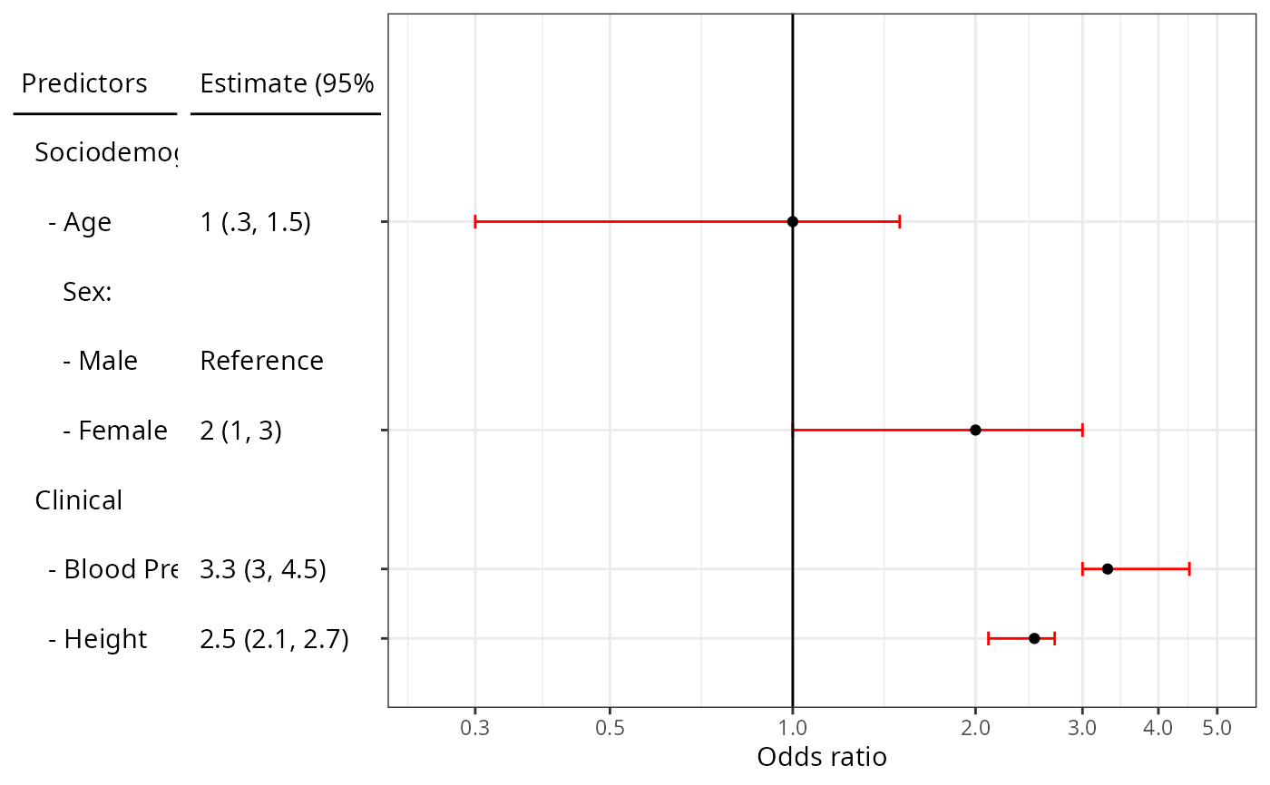
Create a coefficient/model/forest plot
plot_model.RdCreate a coefficient/model/forest plot. I wasn't satisfied with other solutions already floating around, so put this together. It requires some manual intervention but can produce a nice result.
Usage
plot_model(
  df,
  vline = NULL,
  xlab = NULL,
  xbreaks = scales::pretty_breaks(),
  xlim = NULL,
  trans = "identity",
  theme = ggplot2::theme_bw(),
  rel_widths = c(0.15, 0.15, 0.7),
  colname_lines = c(-0.45, NA)
)
Arguments
- df
A data.frame of model results. It must contain the following columns:
predictor- Fill with character vector of predictor variable names.estimate_label- Fill with character vector of coefficient estimates and CI values.estimate- Fill with numeric vector of coefficient estimates.lower- Fill with numeric vector of coefficient lower CI estimates.upper- Fill with numeric vector of coefficient upper CI estimates.
- vline
An integer for the location of the vertical line related to hypothesis test for coefficients.
- xlab
A character string for the x-axis label.
- xbreaks
A numeric vector of x-axis breaks. (passed to
scale_x_continuous())- xlim
A numeric vector (length 2) for the x-axis limits. (passed to
scale_x_continuous())- trans
A string for the transformation to apply to the x-axis. Usually want
"identity"or"log". See?ggplot2::scale_x_continuousfor more information.- theme
ggplot2 theme.
- rel_widths
A numeric vector for the relative widths of the 3 plots that form the final plot.
- colname_lines
A numeric vector of 2 values. Controls the position of the horizontal column name under lines.
Examples
#----------------------------------------------------------------------------
# plot_model() examples
#----------------------------------------------------------------------------
library(bkstat)

df <- data.frame(
predictor = c(
  "Predictors",
  "  Sociodemographic",
  "    - Age",
  "      Sex:",
  "      - Male",
  "      - Female",
  "  Clinical",
  "    - Blood Pressure",
  "    - Height"),
estimate_label = c(
  "Estimate (95% CI)",
  NA,
  "1 (.3, 1.5)",
  NA,
  "Reference",
  "2 (1, 3)",
  NA,
  "3.3 (3, 4.5)",
  "2.5 (2.1, 2.7)"
),
estimate = c(NA, NA, 1, NA, NA, 2, NA, 3.3, 2.5),
lower = c(NA, NA, .3, NA, NA, 1, NA, 3, 2.1),
upper = c(NA, NA, 1.5, NA, NA, 3, NA, 4.5, 2.7)
)

plot_model(
  df = df,
  vline = 1,
  xlab = "Odds ratio",
  xbreaks = c(0.3, 0.5, 1, 2, 3, 4, 5),
  xlim = c(0.25, 5),
  trans = "log"
 )
#> Warning: Removed 9 rows containing missing values or values outside the scale range
#> (`geom_hline()`).
#> Warning: Removed 3 rows containing missing values or values outside the scale range
#> (`geom_text()`).
#> Warning: Removed 9 rows containing missing values or values outside the scale range
#> (`geom_hline()`).
#> `height` was translated to `width`.
#> Warning: Removed 5 rows containing missing values or values outside the scale range
#> (`geom_point()`).