Get the survival probability at a given time
surv_prob.RdThis function has been superseded by bkstat::predict_surv_prob.
Get the survival probability at a given time. A wrapper for survival:::summary.survfit().
Examples
#----------------------------------------------------------------------------
# surv_prob() examples.
#----------------------------------------------------------------------------
library(survival)
library(bkstat)
plot(survfit(formula = Surv(futime, death) ~ trt, data = myeloid))
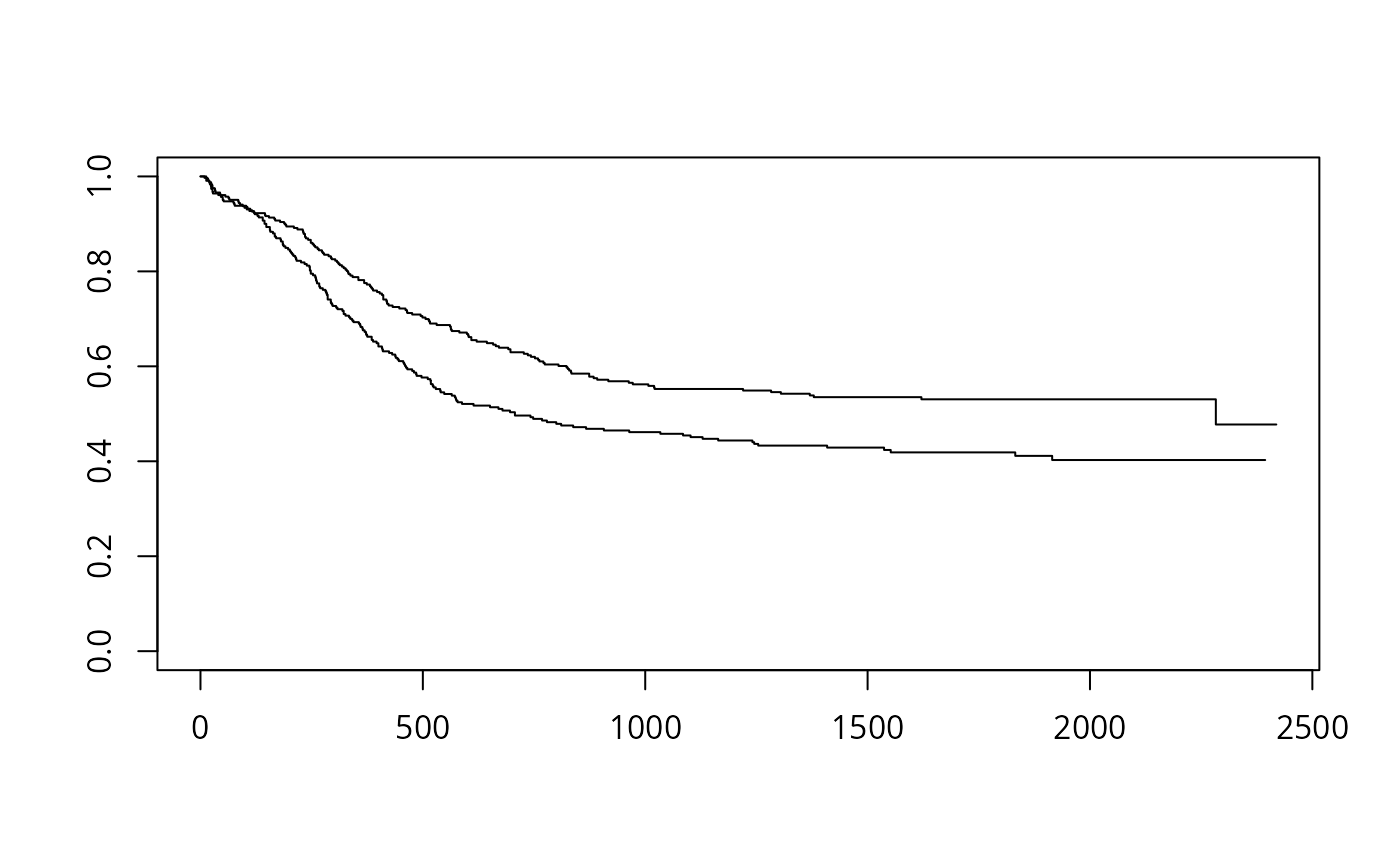 surv_prob(
df = myeloid,
formula = Surv(futime, death) ~ trt,
times = c(100, 500, 2000)
)
#> strata time n n_at_risk n_events n_censored surv_prob lower_ci upper_ci
#> 1 trt=A 100 317 277 20 20 0.9338742 0.9062728 0.9623161
#> 2 trt=A 500 317 167 105 5 0.5764415 0.5226442 0.6357763
#> 3 trt=A 2000 317 38 46 83 0.4026241 0.3473989 0.4666283
#> 4 trt=B 100 329 302 20 7 0.9382070 0.9123374 0.9648102
#> 5 trt=B 500 329 222 75 5 0.7027906 0.6543967 0.7547632
#> 6 trt=B 2000 329 49 53 120 0.5305176 0.4778832 0.5889493
#> ci_level ci_type
#> 1 0.95 log
#> 2 0.95 log
#> 3 0.95 log
#> 4 0.95 log
#> 5 0.95 log
#> 6 0.95 log
surv_prob(
df = myeloid,
formula = Surv(futime, death) ~ 1,
times = c(100, 500, 2000)
)
#> strata time n n_at_risk n_events n_censored surv_prob lower_ci upper_ci
#> 1 Overall 100 646 579 40 27 0.9361388 0.9171812 0.9554883
#> 2 Overall 500 646 389 180 10 0.6422112 0.6053763 0.6812874
#> 3 Overall 2000 646 87 99 203 0.4691332 0.4299483 0.5118894
#> ci_level ci_type
#> 1 0.95 log
#> 2 0.95 log
#> 3 0.95 log
surv_prob(
df = myeloid,
formula = Surv(futime, death) ~ trt + sex,
times = c(100, 500, 2000)
)
#> strata time n n_at_risk n_events n_censored surv_prob lower_ci
#> 1 trt=A, sex=f 100 189 164 9 16 0.9495725 0.9179883
#> 2 trt=A, sex=f 500 189 105 56 3 0.6225603 0.5540913
#> 3 trt=A, sex=f 2000 189 29 24 52 0.4673843 0.3950737
#> 4 trt=A, sex=m 100 128 113 11 4 0.9117194 0.8632355
#> 5 trt=A, sex=m 500 128 62 49 2 0.5119349 0.4306712
#> 6 trt=A, sex=m 2000 128 9 22 31 0.3109665 0.2343301
#> 7 trt=B, sex=f 100 172 159 10 3 0.9411765 0.9064629
#> 8 trt=B, sex=f 500 172 108 47 4 0.6580567 0.5897754
#> 9 trt=B, sex=f 2000 172 28 24 56 0.5064618 0.4349031
#> 10 trt=B, sex=m 100 157 143 10 4 0.9349196 0.8967147
#> 11 trt=B, sex=m 500 157 114 28 1 0.7511892 0.6856341
#> 12 trt=B, sex=m 2000 157 21 29 64 0.5568278 0.4828245
#> upper_ci ci_level ci_type
#> 1 0.9822433 0.95 log
#> 2 0.6994900 0.95 log
#> 3 0.5529299 0.95 log
#> 4 0.9629263 0.95 log
#> 5 0.6085323 0.95 log
#> 6 0.4126666 0.95 log
#> 7 0.9772195 0.95 log
#> 8 0.7342433 0.95 log
#> 9 0.5897946 0.95 log
#> 10 0.9747523 0.95 log
#> 11 0.8230121 0.95 log
#> 12 0.6421737 0.95 log
surv_prob(
df = myeloid,
formula = Surv(futime, death) ~ trt,
times = c(100, 500, 2000)
)
#> strata time n n_at_risk n_events n_censored surv_prob lower_ci upper_ci
#> 1 trt=A 100 317 277 20 20 0.9338742 0.9062728 0.9623161
#> 2 trt=A 500 317 167 105 5 0.5764415 0.5226442 0.6357763
#> 3 trt=A 2000 317 38 46 83 0.4026241 0.3473989 0.4666283
#> 4 trt=B 100 329 302 20 7 0.9382070 0.9123374 0.9648102
#> 5 trt=B 500 329 222 75 5 0.7027906 0.6543967 0.7547632
#> 6 trt=B 2000 329 49 53 120 0.5305176 0.4778832 0.5889493
#> ci_level ci_type
#> 1 0.95 log
#> 2 0.95 log
#> 3 0.95 log
#> 4 0.95 log
#> 5 0.95 log
#> 6 0.95 log
surv_prob(
df = myeloid,
formula = Surv(futime, death) ~ 1,
times = c(100, 500, 2000)
)
#> strata time n n_at_risk n_events n_censored surv_prob lower_ci upper_ci
#> 1 Overall 100 646 579 40 27 0.9361388 0.9171812 0.9554883
#> 2 Overall 500 646 389 180 10 0.6422112 0.6053763 0.6812874
#> 3 Overall 2000 646 87 99 203 0.4691332 0.4299483 0.5118894
#> ci_level ci_type
#> 1 0.95 log
#> 2 0.95 log
#> 3 0.95 log
surv_prob(
df = myeloid,
formula = Surv(futime, death) ~ trt + sex,
times = c(100, 500, 2000)
)
#> strata time n n_at_risk n_events n_censored surv_prob lower_ci
#> 1 trt=A, sex=f 100 189 164 9 16 0.9495725 0.9179883
#> 2 trt=A, sex=f 500 189 105 56 3 0.6225603 0.5540913
#> 3 trt=A, sex=f 2000 189 29 24 52 0.4673843 0.3950737
#> 4 trt=A, sex=m 100 128 113 11 4 0.9117194 0.8632355
#> 5 trt=A, sex=m 500 128 62 49 2 0.5119349 0.4306712
#> 6 trt=A, sex=m 2000 128 9 22 31 0.3109665 0.2343301
#> 7 trt=B, sex=f 100 172 159 10 3 0.9411765 0.9064629
#> 8 trt=B, sex=f 500 172 108 47 4 0.6580567 0.5897754
#> 9 trt=B, sex=f 2000 172 28 24 56 0.5064618 0.4349031
#> 10 trt=B, sex=m 100 157 143 10 4 0.9349196 0.8967147
#> 11 trt=B, sex=m 500 157 114 28 1 0.7511892 0.6856341
#> 12 trt=B, sex=m 2000 157 21 29 64 0.5568278 0.4828245
#> upper_ci ci_level ci_type
#> 1 0.9822433 0.95 log
#> 2 0.6994900 0.95 log
#> 3 0.5529299 0.95 log
#> 4 0.9629263 0.95 log
#> 5 0.6085323 0.95 log
#> 6 0.4126666 0.95 log
#> 7 0.9772195 0.95 log
#> 8 0.7342433 0.95 log
#> 9 0.5897946 0.95 log
#> 10 0.9747523 0.95 log
#> 11 0.8230121 0.95 log
#> 12 0.6421737 0.95 log