Simulate log-transformed lognormal data
sim_log_lognormal.RdSimulate data from the log-transformed lognormal distribution (i.e. a normal distribution) for three scenarios:
One-sample data
Dependent two-sample data
Independent two-sample data
Usage
sim_log_lognormal(
  n1,
  n2 = NULL,
  ratio,
  cv1,
  cv2 = NULL,
  cor = 0,
  nsims = 1L,
  return_type = "list",
  messages = TRUE
)
Arguments
- n1
(integer:
[2, Inf))
The sample size(s) of sample 1.- n2
(integer:
NULL;[2, Inf))
The sample size(s) of sample 2. Set asNULLif you want to simulate for the one-sample case.- ratio
(numeric:
(0, Inf))
The assumed population fold change(s) of sample 2 with respect to sample 1.For one-sample data,
ratiois defined as the geometric mean (GM) of the original lognormal population distribution.For dependent two-sample data,
ratiois defined by GM(sample 2 / sample 1) of the original lognormal population distributions.e.g.
ratio = 2assumes that the geometric mean of all paired ratios (sample 2 / sample 1) is 2.
For independent two-sample data, the
ratiois defined by GM(group 2) / GM(group 1) of the original lognormal population distributions.e.g.
ratio = 2assumes that the geometric mean of sample 2 is 2 times larger than the geometric mean of sample 1.
See 'Details' for additional information.
- cv1
(numeric:
(0, Inf))
The coefficient of variation(s) of sample 1 in the original lognormal data.- cv2
(numeric:
NULL;(0, Inf))
The coefficient of variation(s) of sample 2 in the original lognormal data. Set asNULLif you want to simulate for the one-sample case.- cor
(numeric:
0;[-1, 1])
The correlation(s) between sample 1 and sample 2 in the original lognormal data. Not used for the one-sample case. See 'Details' for constraints based on cv1 and cv2.- nsims
(Scalar integer:
1L;[1,Inf))
The number of simulated data sets. Ifnsims > 1, the data is returned in a list-column of a depower simulation data frame.- return_type
(string:
"list";c("list", "data.frame"))
The data structure of the simulated data. If"list"(default), a list object is returned. If"data.frame"a data frame in tall format is returned. The list object provides computational efficiency and the data frame object is convenient for formulas. See 'Value'.- messages
(Scalar logical:
TRUE)
Whether or not to display messages for pathological simulation cases.
Value
If nsims = 1 and the number of unique parameter combinations is one, the following objects are returned:
If one-sample data with
return_type = "list", a list:Slot Name Description 1 One sample of simulated normal values. If one-sample data with
return_type = "data.frame", a data frame:Column Name Description 1 itemPair/subject/item indicator. 2 valueSimulated normal values. If two-sample data with
return_type = "list", a list:Slot Name Description 1 Simulated normal values from sample 1. 2 Simulated normal values from sample 2. If two-sample data with
return_type = "data.frame", a data frame:Column Name Description 1 itemPair/subject/item indicator. 2 conditionTime/group/condition indicator. 3 valueSimulated normal values.
If nsims > 1 or the number of unique parameter combinations is greater than one, each object described above is returned in data frame, located in a list-column named data.
If one-sample data, a data frame:
Column Name Description 1 n1The sample size. 2 ratioGeometric mean [GM(sample 1)]. 3 cv1Coefficient of variation for sample 1. 4 nsimsNumber of data simulations. 5 distributionDistribution sampled from. 6 dataList-column of simulated data. If two-sample data, a data frame:
Column Name Description 1 n1Sample size of sample 1. 2 n2Sample size of sample 2. 3 ratioRatio of geometric means [GM(sample 2) / GM(sample 1)] or geometric mean ratio [GM(sample 2 / sample 1)]. 4 cv1Coefficient of variation for sample 1. 5 cv2Coefficient of variation for sample 2. 6 corCorrelation between samples. 7 nsimsNumber of data simulations. 8 distributionDistribution sampled from. 9 dataList-column of simulated data.
Details
Based on assumed characteristics of the original lognormal distribution, data is simulated from the corresponding log-transformed (normal) distribution. This simulated data is suitable for assessing power of a hypothesis for the geometric mean or ratio of geometric means from the original lognormal data.
This method can also be useful for other population distributions which are positive and where it makes sense to describe the ratio of geometric means. However, the lognormal distribution is theoretically correct in the sense that you can log-transform to a normal distribution, compute the summary statistic, then apply the inverse transformation to summarize on the original lognormal scale.
Notation
| Symbol | Definition |
| \(GM(\cdot)\) | Geometric mean |
| \(AM(\cdot)\) | Arithmetic mean |
| \(CV(\cdot)\) | Coefficient of variation |
| \(\sigma^2\) | Variance |
| \(\rho\) | Correlation |
| \(\ln\) | Natural Log |
| \(X_i\) | Lognormal random variable for group \(i\) |
| \(Y_i\) | Log-transformed lognormal random variable for group \(i\) |
Fold Change and the Ratio Parameter
The ratio parameter (fold change) is defined as follows for each scenario:
One-sample: \(\text{ratio} = GM(X)\)
Dependent two-sample: \(\text{ratio} = GM \left( \frac{X_2}{X_1} \right)\)
Independent two-sample: \(\text{ratio} = \frac{GM(X_2)}{GM(X_1)}\)
For equal sample sizes of \(X_1\) and \(X_2\), these definitions are connected by the identity
$$ \begin{aligned} \frac{GM(X_2)}{GM(X_1)} &= GM\left( \frac{X_2}{X_1} \right) \\ &= e^{AM(Y_2) - AM(Y_1)} \\ &= e^{AM(Y_2 - Y_1)}. \end{aligned} $$
Coefficient of Variation
The coefficient of variation (CV) for a random variable \(X\) is defined as
$$CV(X) = \frac{\sigma_{X}}{AM(X)}.$$
Relationships Between Original and Log Scales
The following relationships allow conversion between scales.
From log scale to original lognormal scale:
$$ \begin{aligned} AM(X) &= e^{AM(Y) + \sigma^2_Y / 2} \\ GM(X) &= e^{AM(Y)} \\ \sigma^2_{X} &= AM(X)^2 \left( e^{\sigma^2_Y} - 1 \right) \\ CV(X) &= \frac{\sqrt{AM(X)^2 \left( e^{\sigma^2_Y} - 1 \right)}}{AM(X)} \\ &= \sqrt{e^{\sigma^2_Y} - 1}. \end{aligned} $$
From original lognormal scale to log scale:
$$ \begin{aligned} AM(Y) &= \ln \left( \frac{AM(X)}{\sqrt{CV(X)^2 + 1}} \right) \\ \sigma^2_Y &= \ln(CV(X)^2 + 1) \\ \rho_{Y_1, Y_2} &= \frac{\ln \left( \rho_{X_1, X_2}CV(X_1)CV(X_2) + 1 \right)}{\sqrt{\ln(CV(X_1)^2 + 1)}\sqrt{\ln(CV(X_2)^2 + 1)}} \\ &= \frac{\ln \left( \rho_{X_1, X_2}CV(X_1)CV(X_2) + 1 \right)}{\sigma_{Y_1}\sigma_{Y_2}}. \end{aligned} $$
Dependent Samples
Correlation Constraints
Not all combinations of cor, cv1, and cv2 yield a valid correlation on the log scale.
Two constraints must be satisfied.
First, the logarithm argument must be positive:
$$ \rho_{X_1, X_2} \cdot CV(X_1) \cdot CV(X_2) + 1 > 0 $$
which implies
$$ \rho_{X_1, X_2} > \frac{-1}{CV(X_1) \cdot CV(X_2)}. $$
Second, the log-scale correlation must be in \((-1, 1)\):
$$ \frac{e^{-\sigma_{Y_1} \sigma_{Y_2}} - 1}{CV(X_1) \cdot CV(X_2)} < \rho_{X_1, X_2} < \frac{e^{\sigma_{Y_1} \sigma_{Y_2}} - 1}{CV(X_1) \cdot CV(X_2)}. $$
The lower bound of the second constraint is always more restrictive than the first constraint, so the second constraint is sufficient.
When \(CV(X_1) = CV(X_2) = CV\), the second constraint simplifies to:
$$ \frac{-1}{CV^2 + 1} < \rho_{X_1, X_2} < 1 $$
For equal CVs, only negative correlations are constrained.
For example, with \(CV = 0.5\), the valid range for cor is approximately \((-0.80, 1)\).
When \(CV(X_1) \neq CV(X_2)\), both bounds may be constrained.
The upper bound is strictly less than 1, meaning even positive correlations near 1 can be infeasible.
For example, with \(CV(X_1) = 0.1\) and \(CV(X_2) = 1\), the valid range for cor is approximately \((-0.80, 0.87)\).
Equivalent One-Sample Representation
Two-sample dependent data can be represented as an equivalent paired one-sample problem. First, consider the properties of variance and covariance. The variance of the difference between two dependent samples on the log scale (normal distribution) is:
$$ \begin{aligned} \sigma^2_{Y_2 - Y_1} &= \sigma^2_{Y_1} + \sigma^2_{Y_2} - 2 Cov(Y_1, Y_2) \\ &= \sigma^2_{Y_1} + \sigma^2_{Y_2} - 2 \rho_{Y_1, Y_2} \sigma_{Y_1} \sigma_{Y_2} \end{aligned} $$
Positive correlation reduces the variance of differences, while negative correlation increases it. For the special case where the two samples are uncorrelated and have equal variance: \(\sigma^2_{Y_2 - Y_1} = 2\sigma^2\).
Second, substitute \(\rho\) and \(\sigma^2\) with their alternative forms:
$$ \begin{aligned} \sigma^2_{Y_2 - Y_1} &= \sigma^2_{Y_1} + \sigma^2_{Y_2} - 2 \rho_{Y_1, Y_2} \sigma_{Y_1} \sigma_{Y_2} \\ &= \ln(CV(X_1)^2 + 1) + \ln(CV(X_2)^2 + 1) - 2\ln(\rho_{X_1, X_2}CV(X_1)CV(X_2) + 1) \\ &= \ln\left(\frac{(CV(X_1)^2 + 1)(CV(X_2)^2 + 1)}{(\rho_{X_1, X_2}CV(X_1)CV(X_2) + 1)^2}\right). \end{aligned} $$
Finally, denote log-transformed one-sample paired difference as \(Y_{\text{diff}}\). It follows that \(\sigma^2_{Y_{\text{diff}}} = \ln(CV(X_{\text{diff}})^2 + 1)\). We need to solve for \(CV(X_{\text{diff}})\) so that the variance of the log-transformed one-sample values match the variance of the log-transformed two-sample differences. This results in
$$ CV(X_{\text{diff}}) = \sqrt{\frac{(CV(X_1)^2 + 1)(CV(X_2)^2 + 1)}{(\rho_{X_1, X_2}CV(X_1)CV(X_2) + 1)^2} - 1} $$
When \(CV(X_1) = CV(X_2) = CV\), this simplifies to
$$ CV(X_{\text{diff}}) = \sqrt{\left( \frac{CV^2 + 1}{\rho_{X_1, X_2} CV^2 + 1} \right)^2 - 1} $$
This equivalence allows dependent two-sample data to be simulated (with lognormal scale arguments cv1, cv2, and cor) using a one-sample simulation (with lognormal scale argument cv1).
References
Julious SA (2004). “Sample sizes for clinical trials with Normal data.” Statistics in Medicine, 23(12), 1921–1986. doi:10.1002/sim.1783 .
Hauschke D, Steinijans VW, Diletti E, Burke M (1992). “Sample size determination for bioequivalence assessment using a multiplicative model.” Journal of Pharmacokinetics and Biopharmaceutics, 20(5), 557–561. ISSN 0090-466X, doi:10.1007/BF01061471 .
Johnson NL, Kotz S, Balakrishnan N (1994). Continuous univariate distributions, Wiley series in probability and mathematical statistics, 2nd ed edition. Wiley, New York. ISBN 9780471584957 9780471584940.
Examples
#----------------------------------------------------------------------------
# sim_log_lognormal() examples
#----------------------------------------------------------------------------
library(depower)
# Independent two-sample data returned in a data frame
sim_log_lognormal(
n1 = 10,
n2 = 10,
ratio = 1.3,
cv1 = 0.35,
cv2 = 0.35,
cor = 0,
nsims = 1,
return_type = "data.frame"
)
#> item condition value
#> 1 1 1 0.4374262058
#> 2 2 1 0.1804416333
#> 3 3 1 -0.8747521366
#> 4 4 1 0.2086864433
#> 5 5 1 0.0735927903
#> 6 6 1 0.4691575138
#> 7 7 1 0.2245717051
#> 8 8 1 -0.0181373206
#> 9 9 1 -0.0009699646
#> 10 10 1 -0.0567030643
#> 11 1 2 0.3275196974
#> 12 2 2 0.4989171286
#> 13 3 2 -0.2235746903
#> 14 4 2 0.4614657690
#> 15 5 2 0.6641219751
#> 16 6 2 0.3462268592
#> 17 7 2 0.6782718413
#> 18 8 2 0.3224740428
#> 19 9 2 0.5958203692
#> 20 10 2 0.3210771127
# Independent two-sample data returned in a list
sim_log_lognormal(
n1 = 10,
n2 = 10,
ratio = 1.3,
cv1 = 0.35,
cv2 = 0.35,
cor = 0,
nsims = 1,
return_type = "list"
)
#> $value1
#> [1] -0.49306243 -0.36245087 -0.19180040 0.07295877 -0.22441038 0.22036359
#> [7] -0.36602551 -0.20025322 -0.08099939 0.31799241
#>
#> $value2
#> [1] -0.25876051 0.28413884 0.07704966 0.19024698 0.02223258 0.39304949
#> [7] 0.27707842 0.39992326 0.07236936 0.31561467
#>
# Dependent two-sample data returned in a data frame
sim_log_lognormal(
n1 = 10,
n2 = 10,
ratio = 1.3,
cv1 = 0.35,
cv2 = 0.35,
cor = 0.4,
nsims = 1,
return_type = "data.frame"
)
#> item condition value
#> 1 1 1 -0.30537250
#> 2 2 1 0.30143341
#> 3 3 1 0.35767885
#> 4 4 1 0.48329177
#> 5 5 1 0.05529636
#> 6 6 1 -0.48936821
#> 7 7 1 0.25331762
#> 8 8 1 0.24241776
#> 9 9 1 -0.14187633
#> 10 10 1 -0.11429514
#> 11 1 2 0.33760424
#> 12 2 2 0.43157328
#> 13 3 2 0.54794127
#> 14 4 2 0.96732708
#> 15 5 2 -0.06264886
#> 16 6 2 -0.12696981
#> 17 7 2 0.53968991
#> 18 8 2 0.14669384
#> 19 9 2 0.34354843
#> 20 10 2 -0.09255898
# Dependent two-sample data returned in a list
sim_log_lognormal(
n1 = 10,
n2 = 10,
ratio = 1.3,
cv1 = 0.35,
cv2 = 0.35,
cor = 0.4,
nsims = 1,
return_type = "list"
)
#> $value1
#> [1] 0.093052221 0.007403719 -0.075171464 0.330256224 0.023824239
#> [6] 0.376068817 0.004727940 -0.048544341 0.631188589 0.361732038
#>
#> $value2
#> [1] 0.61918575 0.34492199 0.65338363 -0.03767743 -0.02549460 0.41548563
#> [7] 0.58917893 0.23717366 0.14135692 -0.08237838
#>
# One-sample data returned in a data frame
sim_log_lognormal(
n1 = 10,
ratio = 1.3,
cv1 = 0.35,
nsims = 1,
return_type = "data.frame"
)
#> item value
#> 1 1 0.56535871
#> 2 2 0.50327718
#> 3 3 0.34817855
#> 4 4 0.44742367
#> 5 5 -0.01076548
#> 6 6 -0.36891047
#> 7 7 0.22727584
#> 8 8 0.53228901
#> 9 9 0.22009162
#> 10 10 0.28968503
# One-sample data returned in a list
sim_log_lognormal(
n1 = 10,
ratio = 1.3,
cv1 = 0.35,
nsims = 1,
return_type = "list"
)
#> $value1
#> [1] -0.0339542 0.1515314 0.1195203 0.5489847 0.2128871 -0.3116690
#> [7] 1.2097556 0.4490520 0.2514237 0.5276685
#>
# Independent two-sample data: two simulations for four parameter combinations.
# Returned as a list-column of lists within a data frame
sim_log_lognormal(
n1 = c(10, 20),
n2 = c(10, 20),
ratio = 1.3,
cv1 = 0.35,
cv2 = 0.35,
cor = 0,
nsims = 2,
return_type = "list"
)
#> # A tibble: 4 × 9
#> n1 n2 ratio cv1 cv2 cor nsims distribution data
#> <dbl> <dbl> <dbl> <dbl> <dbl> <dbl> <dbl> <chr> <list>
#> 1 10 10 1.3 0.35 0.35 0 2 Independent two-sample log(l… <list>
#> 2 20 10 1.3 0.35 0.35 0 2 Independent two-sample log(l… <list>
#> 3 10 20 1.3 0.35 0.35 0 2 Independent two-sample log(l… <list>
#> 4 20 20 1.3 0.35 0.35 0 2 Independent two-sample log(l… <list>
# Dependent two-sample data: two simulations for two parameter combinations.
# Returned as a list-column of lists within a data frame
sim_log_lognormal(
n1 = c(10, 20),
n2 = c(10, 20),
ratio = 1.3,
cv1 = 0.35,
cv2 = 0.35,
cor = 0.4,
nsims = 2,
return_type = "list"
)
#> # A tibble: 2 × 9
#> n1 n2 ratio cv1 cv2 cor nsims distribution data
#> <dbl> <dbl> <dbl> <dbl> <dbl> <dbl> <dbl> <chr> <list>
#> 1 10 10 1.3 0.35 0.35 0.4 2 Dependent two-sample log(log… <list>
#> 2 20 20 1.3 0.35 0.35 0.4 2 Dependent two-sample log(log… <list>
# One-sample data: two simulations for two parameter combinations
# Returned as a list-column of lists within a data frame
sim_log_lognormal(
n1 = c(10, 20),
ratio = 1.3,
cv1 = 0.35,
nsims = 2,
return_type = "list"
)
#> # A tibble: 2 × 6
#> n1 ratio cv1 nsims distribution data
#> <dbl> <dbl> <dbl> <dbl> <chr> <list>
#> 1 10 1.3 0.35 2 One-sample log(lognormal) <list [2]>
#> 2 20 1.3 0.35 2 One-sample log(lognormal) <list [2]>
#----------------------------------------------------------------------------
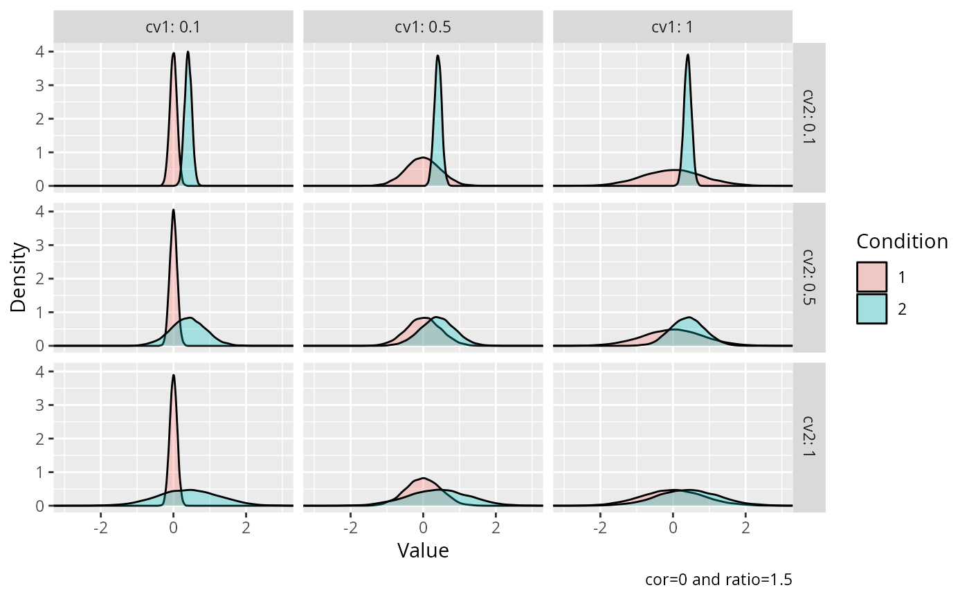
# Visualization of independent two-sample data from a log-transformed
# lognormal distribution with varying coefficient of variation.
#----------------------------------------------------------------------------
cv <- expand.grid(c(0.1, 0.5, 1), c(0.1, 0.5, 1))
set.seed(1234)
data <- mapply(
FUN = function(cv1, cv2) {
d <- sim_log_lognormal(
n1 = 10000,
n2 = 10000,
ratio = 1.5,
cv1 = cv1,
cv2 = cv2,
cor = 0,
nsims = 1,
return_type = "data.frame"
)
cbind(cv1 = cv1, cv2 = cv2, d)
},
cv1 = cv[[1]],
cv2 = cv[[2]],
SIMPLIFY = FALSE
)
data <- do.call(what = "rbind", args = data)
ggplot2::ggplot(
data = data,
mapping = ggplot2::aes(x = value, fill = condition)
) +
ggplot2::facet_grid(
rows = ggplot2::vars(.data$cv2),
cols = ggplot2::vars(.data$cv1),
labeller = ggplot2::labeller(
.rows = ggplot2::label_both,
.cols = ggplot2::label_both
)
) +
ggplot2::geom_density(alpha = 0.3) +
ggplot2::coord_cartesian(xlim = c(-3, 3)) +
ggplot2::labs(
x = "Value",
y = "Density",
fill = "Condition",
caption = "cor=0 and ratio=1.5"
)
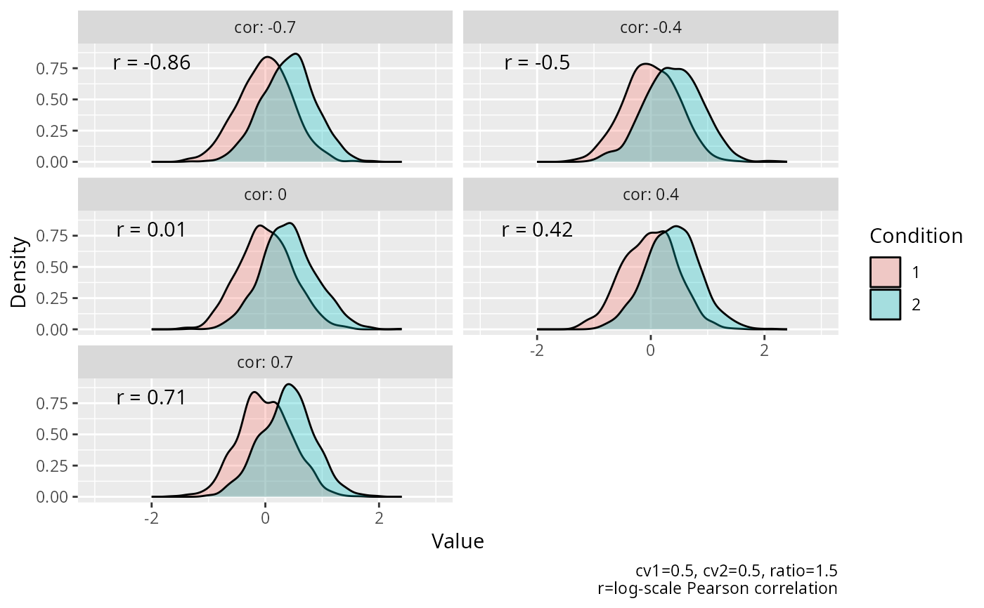
 #----------------------------------------------------------------------------
# Visualization of dependent two-sample data from a log-transformed lognormal
# distribution with varying correlation.
# The first figure shows the marginal distribution for each group.
# The second figure shows the joint distribution for each group.
# The third figure shows the distribution of differences.
#----------------------------------------------------------------------------
set.seed(1234)
data <- lapply(
X = c(-0.7, -0.4, 0, 0.4, 0.7),
FUN = function(x) {
d <- sim_log_lognormal(
n1 = 1000,
n2 = 1000,
cv1 = 0.5,
cv2 = 0.5,
ratio = 1.5,
cor = x,
nsims = 1,
return_type = "data.frame"
)
cor <- cor(
x = d[d$condition == 1, ]$value,
y = d[d$condition == 2, ]$value
)
cbind(cor = x, r = cor, d)
}
)
data <- do.call(what = "rbind", args = data)
# Density plot of marginal distributions
ggplot2::ggplot(
data = data,
mapping = ggplot2::aes(x = value, fill = condition)
) +
ggplot2::facet_wrap(
facets = ggplot2::vars(.data$cor),
ncol = 2,
labeller = ggplot2::labeller(.rows = ggplot2::label_both)
) +
ggplot2::geom_density(alpha = 0.3) +
ggplot2::coord_cartesian(xlim = c(-3, 3)) +
ggplot2::geom_text(
mapping = ggplot2::aes(
x = -2,
y = 0.8,
label = paste0("r = ", round(r, 2))
),
check_overlap = TRUE
) +
ggplot2::labs(
x = "Value",
y = "Density",
fill = "Condition",
caption = "cv1=0.5, cv2=0.5, ratio=1.5\nr=log-scale Pearson correlation"
)
#----------------------------------------------------------------------------
# Visualization of dependent two-sample data from a log-transformed lognormal
# distribution with varying correlation.
# The first figure shows the marginal distribution for each group.
# The second figure shows the joint distribution for each group.
# The third figure shows the distribution of differences.
#----------------------------------------------------------------------------
set.seed(1234)
data <- lapply(
X = c(-0.7, -0.4, 0, 0.4, 0.7),
FUN = function(x) {
d <- sim_log_lognormal(
n1 = 1000,
n2 = 1000,
cv1 = 0.5,
cv2 = 0.5,
ratio = 1.5,
cor = x,
nsims = 1,
return_type = "data.frame"
)
cor <- cor(
x = d[d$condition == 1, ]$value,
y = d[d$condition == 2, ]$value
)
cbind(cor = x, r = cor, d)
}
)
data <- do.call(what = "rbind", args = data)
# Density plot of marginal distributions
ggplot2::ggplot(
data = data,
mapping = ggplot2::aes(x = value, fill = condition)
) +
ggplot2::facet_wrap(
facets = ggplot2::vars(.data$cor),
ncol = 2,
labeller = ggplot2::labeller(.rows = ggplot2::label_both)
) +
ggplot2::geom_density(alpha = 0.3) +
ggplot2::coord_cartesian(xlim = c(-3, 3)) +
ggplot2::geom_text(
mapping = ggplot2::aes(
x = -2,
y = 0.8,
label = paste0("r = ", round(r, 2))
),
check_overlap = TRUE
) +
ggplot2::labs(
x = "Value",
y = "Density",
fill = "Condition",
caption = "cv1=0.5, cv2=0.5, ratio=1.5\nr=log-scale Pearson correlation"
)
 # Reshape to wide format for scatterplot
data_wide <- data.frame(
cor = data[data$condition == "1", ]$cor,
r = data[data$condition == "1", ]$r,
value1 = data[data$condition == "1", ]$value,
value2 = data[data$condition == "2", ]$value
)
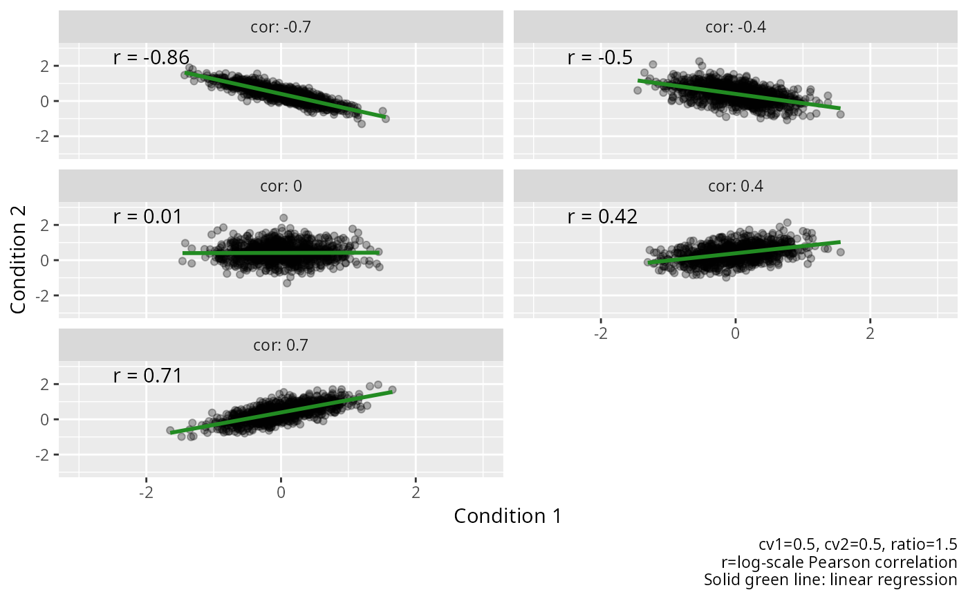
# Scatterplot of joint distribution
ggplot2::ggplot(
data = data_wide,
mapping = ggplot2::aes(x = value1, y = value2)
) +
ggplot2::facet_wrap(
facets = ggplot2::vars(.data$cor),
ncol = 2,
labeller = ggplot2::labeller(.rows = ggplot2::label_both)
) +
ggplot2::geom_point(alpha = 0.3) +
ggplot2::geom_smooth(
method = "lm",
se = FALSE,
color = "forestgreen"
) +
ggplot2::geom_text(
data = unique(data_wide[c("cor", "r")]),
mapping = ggplot2::aes(
x = -2.5,
y = 2.5,
label = paste0("r = ", round(r, 2))
),
hjust = 0
) +
ggplot2::coord_cartesian(xlim = c(-3, 3), ylim = c(-3, 3)) +
ggplot2::labs(
x = "Condition 1",
y = "Condition 2",
caption = paste0(
"cv1=0.5, cv2=0.5, ratio=1.5",
"\nr=log-scale Pearson correlation",
"\nSolid green line: linear regression"
)
)
#> `geom_smooth()` using formula = 'y ~ x'
# Reshape to wide format for scatterplot
data_wide <- data.frame(
cor = data[data$condition == "1", ]$cor,
r = data[data$condition == "1", ]$r,
value1 = data[data$condition == "1", ]$value,
value2 = data[data$condition == "2", ]$value
)
# Scatterplot of joint distribution
ggplot2::ggplot(
data = data_wide,
mapping = ggplot2::aes(x = value1, y = value2)
) +
ggplot2::facet_wrap(
facets = ggplot2::vars(.data$cor),
ncol = 2,
labeller = ggplot2::labeller(.rows = ggplot2::label_both)
) +
ggplot2::geom_point(alpha = 0.3) +
ggplot2::geom_smooth(
method = "lm",
se = FALSE,
color = "forestgreen"
) +
ggplot2::geom_text(
data = unique(data_wide[c("cor", "r")]),
mapping = ggplot2::aes(
x = -2.5,
y = 2.5,
label = paste0("r = ", round(r, 2))
),
hjust = 0
) +
ggplot2::coord_cartesian(xlim = c(-3, 3), ylim = c(-3, 3)) +
ggplot2::labs(
x = "Condition 1",
y = "Condition 2",
caption = paste0(
"cv1=0.5, cv2=0.5, ratio=1.5",
"\nr=log-scale Pearson correlation",
"\nSolid green line: linear regression"
)
)
#> `geom_smooth()` using formula = 'y ~ x'
 # Density plot of differences
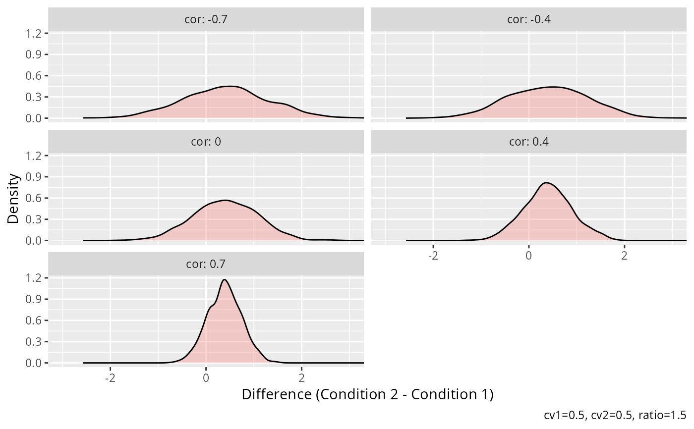
# Paired differences have decreasing variance as correlation increases.
data_wide$difference <- data_wide$value2 - data_wide$value1
ggplot2::ggplot(
data = data_wide,
mapping = ggplot2::aes(x = difference)
) +
ggplot2::facet_wrap(
facets = ggplot2::vars(.data$cor),
ncol = 2,
labeller = ggplot2::labeller(.rows = ggplot2::label_both)
) +
ggplot2::geom_density(alpha = 0.3, fill = "#F8766D") +
ggplot2::coord_cartesian(xlim = c(-3, 3)) +
ggplot2::labs(
x = "Difference (Condition 2 - Condition 1)",
y = "Density",
caption = "cv1=0.5, cv2=0.5, ratio=1.5"
)
# Density plot of differences
# Paired differences have decreasing variance as correlation increases.
data_wide$difference <- data_wide$value2 - data_wide$value1
ggplot2::ggplot(
data = data_wide,
mapping = ggplot2::aes(x = difference)
) +
ggplot2::facet_wrap(
facets = ggplot2::vars(.data$cor),
ncol = 2,
labeller = ggplot2::labeller(.rows = ggplot2::label_both)
) +
ggplot2::geom_density(alpha = 0.3, fill = "#F8766D") +
ggplot2::coord_cartesian(xlim = c(-3, 3)) +
ggplot2::labs(
x = "Difference (Condition 2 - Condition 1)",
y = "Density",
caption = "cv1=0.5, cv2=0.5, ratio=1.5"
)