Weighted hierarchical clustering of variables
build_tree.RdPerforms ascendant hierarchical clustering of variables for quantitative, categorical, or mixed datasets with row weights.
For each candidate cluster, a quantitative synthetic variable is computed as the first component of a weighted factorial method (FactoMineR::FAMD() for mixed data, FactoMineR::PCA() for purely quantitative data, FactoMineR::MCA() for purely categorical data).
The homogeneity of a cluster is defined as the sum, over variables in the cluster, of weighted squared Pearson correlations (for quantitative variables) and weighted squared correlation ratios (\(\eta^2\)) (for categorical variables) with the synthetic variable.
Clusters are agglomerated by minimizing the loss of homogeneity when two clusters are merged, reproducing the methods of ClustOfVar::hclustvar().
Arguments
- data
(data.frame)
Adata.framewith numeric and/or factor columns for clustering. Character columns will be converted to factor. Optionally, including a column of numeric weights. Must not contain missing values.- weights
(Scalar character or
NULL)
Column name of row weights. IfNULL(default), equal weights are used. Weights must be nonnegative, with \(\sum_i w_i > 0\). Zeros are allowed (rows with zero weight contribute nothing).- monotone
(Scalar logical:
FALSE)
Whether or not dendrogram heights should be monotone (to prevent inversions).
Value
A list of class "build_tree" with elements:
merge: Integer matrix of size \((p-1)\times 2\) describing the merge history in hclust convention. Row i of merge describes the merging of clusters at step i of the clustering. If an element j in the row is negative, then variable -j was merged at this stage. If j is positive then the merge was with the cluster formed at the (earlier) stage j of the algorithm. Thus negative entries in merge indicate agglomerations of singletons, and positive entries indicate agglomerations of non-singletons.height: Numeric vector of length \(p-1\) with dissimilarities \(d(A,B) = H(A)+H(B)-H(A\cup B)\) recorded at each merge.order: A vector giving the permutation of the original variables suitable for plotting, in the sense that a cluster plot using this ordering and matrix merge will not have crossings of the branches.labels: Character vector of variable names.clusmat: Integer matrix \(p\times p\) giving cluster memberships of variables at each level (columns correspond to \(k = 1, \dots, p\) clusters, where column j gives the cluster assignment when the tree is cut into j clusters).call: The matched call.data: The data frame of variables used for clustering, including the weight column (if any). The attribute".row.weights"stores the weight column name.method:"build_tree"
The attribute ".row.weights" stores the weight column name.
Details
If missing values are present in your data, you must either impute them or subset to complete cases before analysis. For example,
data_cc <- data[complete.cases(data), ]If variables with zero-variance or less than two factor levels are present in your data, you must exclude them before analysis. For example,
w <- data$weights
valid_vars <- function(x) {
  if(is.numeric(x)) {
    vclust:::weighted_var(x, w) > .Machine$double.eps
  } else if(is.factor(x) || is.character(x) || is.logical(x)) {
    nlevels(droplevels(as.factor(x))) > 1
  } else {
    FALSE
  }
}
are_valid <- vapply(data, valid_vars, logical(1))
data_valid <- data[are_valid]
Let \(\mathbf{x}_1, \dots, \mathbf{x}_{p_1}\) be quantitative variables and \(\mathbf{z}_1, \dots, \mathbf{z}_{p_2}\) be categorical variables measured on \(n\) observations, with \(p = p_1 + p_2\). Denote a candidate cluster of variables as \(C_k\). A partition \(P_K=(C_1, \dots, C_K)\) groups variables into \(K\) clusters. For a given cluster \(C_k\), a quantitative synthetic variable \(\mathbf{y}_k \in \mathbb{R}^n\) is defined as the variable most related to all variables in \(C_k\):
$$ \mathbf{y}_k = \arg\max_{\mathbf{u}\in\mathbb{R}^n} \left\{ \sum_{\mathbf{x}_j \in C_k} r^2(\mathbf{u}, \mathbf{x}_j) \;+\; \sum_{\mathbf{z}_j \in C_k} \eta^2(\mathbf{u}\mid \mathbf{z}_j) \right\}, $$
where \(r^2\) is the weighted squared Pearson correlation and \(\eta^2\) is the weighted squared correlation ratio (the fraction of the variance of \(\mathbf{u}\) explained by the categories of \(\mathbf{z}_j\)).
In the unweighted ClustOfVar::hclustvar() method, \(\mathbf{y}_k\) is the first component of PCAmixdata::PCAmix() on the variables in \(C_k\), and the homogeneity of the cluster equals the first eigenvalue \(\lambda_1^k\) of PCAmixdata::PCAmix().
In this weighted extension, we replace PCAmixdata::PCAmix() using FactoMineR:
FactoMineR::FAMD for mixed clusters,
FactoMineR::PCA for purely quantitative clusters,
FactoMineR::MCA for purely categorical clusters,
each with row weights. The homogeneity is computed as
$$ H(C_k) = \sum_{\mathbf{x}_j \in C_k} r^2(\mathbf{y}_k,\mathbf{x}_j) + \sum_{\mathbf{z}_j \in C_k} \eta^2(\mathbf{y}_k \mid \mathbf{z}_j), $$
where \(\mathbf{y}_k\) is the first‑axis score (res$ind$coord[,1L]) of the corresponding weighted FactoMineR result.
Weighted Measures
Let \(w_i \ge 0\) denote row weights for \(i=1, \dots, n\), normalized to sum to one: \(\tilde{w}_i = w_i / \sum_{j} w_j\). The weighted mean, variance, and covariance are
$$ \bar{x} = \sum_{i=1}^{n} \tilde{w}_i \, x_i, $$
$$ \mathrm{var}_w(x) = \sum_{i=1}^{n} \tilde{w}_i\,(x_i-\bar{x})^2, $$
$$ \mathrm{cov}_w(x,y) = \sum_{i=1}^{n} \tilde{w}_i\,(x_i-\bar{x})(y_i-\bar{y}), $$
and the weighted Pearson correlation is
$$ r_w(x,y) = \frac{\mathrm{cov}_w(x,y)}{\sqrt{\mathrm{var}_w(x)\,\mathrm{var}_w(y)}}. $$
For a numeric variable \(x\) and a factor \(g\) with groups indexed by \(s\), the weighted squared correlation ratio is
$$ \eta^2(x\mid g) = \frac{\mathrm{SSB}}{\mathrm{SST}} = \frac{\sum_{s} W_s \,(\bar{x}_s - \bar{x})^2} {\sum_{i} \tilde{w}_i \,(x_i-\bar{x})^2}, $$
where \(W_s=\sum_{i\in s}\tilde{w}_i\), \(\bar{x}_s=\sum_{i\in s}\tilde{w}_i x_i/W_s\), and \(\bar{x}=\sum_i \tilde{w}_i x_i\).
Agglomeration Criterion
Following ClustOfVar::hclustvar(), the dissimilarity between two clusters \(A\) and \(B\) is the loss of homogeneity when merging:
$$ d(A,B) = H(A) + H(B) - H(A \cup B). $$
At each step, the algorithm merges the pair with the smallest \(d(A,B)\). The dendrogram height recorded for the new node is \(d(A,B)\).
Dendrogram heights
A dendrogram inversion occurs when a merge step records a smaller dissimilarity than a preceding merge step.
In the dendrogram, this appears as a branch that merges at a lower height than its children branches.
Generally, hierarchical clustering should be defined by non-decreasing distances as the algorithm progresses and combines larger clusters.
For plotting stability, a base::cummax() adjustment (via monotone = TRUE) is used to enforce monotone heights.
This adjusts the recorded heights for plotting but does not change the merge order, cluster memberships, or variable ordering.
Dendrogram inversions are rare in practice.
References
Chavent M, Kuentz-Simonet V, Liquet B, Saracco J (2012). “ClustOfVar: An R Package for the Clustering of Variables.” Journal of Statistical Software, 50(13), 1–16. doi:10.18637/jss.v050.i13 , https://www.jstatsoft.org/index.php/jss/article/view/v050i13.
Lê S, Josse J, Husson F (2008). “FactoMineR: A Package for Multivariate Analysis.” Journal of Statistical Software, 25(1), 1–18. doi:10.18637/jss.v025.i01 .
Examples
#----------------------------------------------------------------------------
# build_tree() examples
#----------------------------------------------------------------------------
library(vclust)
# Example 1: Quantitative variables with equal weights
set.seed(42)
n <- 60
data <- data.frame(
col1 = rnorm(n),
col2 = rnorm(n),
col3 = rnorm(n),
col4 = rnorm(n),
weights = rep(1, n)
)
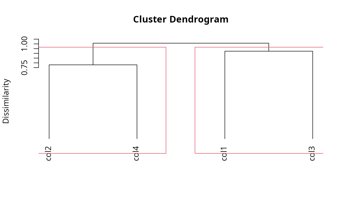
tree <- build_tree(data = data, weights = "weights")
plot(tree)
rect.hclust(tree = tree, k = 2)
 head(tree$merge)
#> [,1] [,2]
#> [1,] -2 -4
#> [2,] -1 -3
#> [3,] 1 2
head(tree$height)
#> [1] 0.7790883 0.9231259 1.0074275
# Example 2: Mixed data with equal weights
set.seed(70)
n <- 80
X <- data.frame(
col1 = rnorm(n),
col2 = rnorm(n) + 0.6*rnorm(n)
)
Z <- data.frame(
col3 = factor(sample(letters[1:3], n, TRUE)),
col4 = factor(sample(c("L","M","H"), n, TRUE))
)
w <- rep(1, n) # equal weights
data <- cbind(X, Z, w)
tree_mix <- build_tree(data = data, weights = "w")
plot(tree_mix)
rect.hclust(tree = tree_mix, k = 2)
head(tree$merge)
#> [,1] [,2]
#> [1,] -2 -4
#> [2,] -1 -3
#> [3,] 1 2
head(tree$height)
#> [1] 0.7790883 0.9231259 1.0074275
# Example 2: Mixed data with equal weights
set.seed(70)
n <- 80
X <- data.frame(
col1 = rnorm(n),
col2 = rnorm(n) + 0.6*rnorm(n)
)
Z <- data.frame(
col3 = factor(sample(letters[1:3], n, TRUE)),
col4 = factor(sample(c("L","M","H"), n, TRUE))
)
w <- rep(1, n) # equal weights
data <- cbind(X, Z, w)
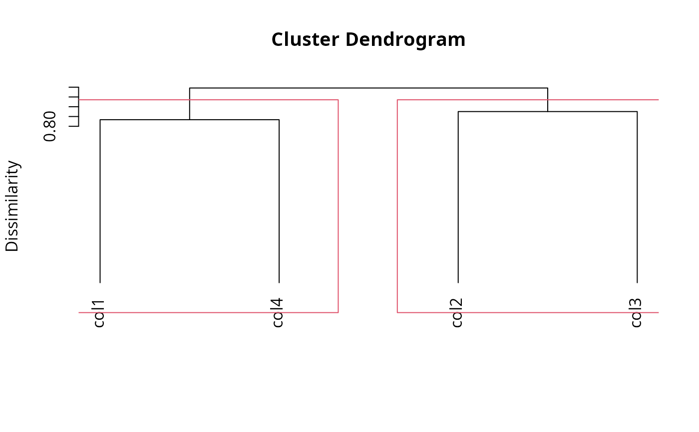
tree_mix <- build_tree(data = data, weights = "w")
plot(tree_mix)
rect.hclust(tree = tree_mix, k = 2)
 head(tree_mix$merge)
#> [,1] [,2]
#> [1,] -1 -4
#> [2,] -2 -3
#> [3,] 1 2
head(tree_mix$height)
#> [1] 0.8337201 0.8753501 0.9958184
# Example 3: Mixed data with unequal weights
set.seed(70)
w <- rexp(n) # positive, exponential weights
data <- cbind(X, Z, w)
tree_mix <- build_tree(data = data, weights = "w")
plot(tree_mix)
rect.hclust(tree = tree_mix, k = 2)
head(tree_mix$merge)
#> [,1] [,2]
#> [1,] -1 -4
#> [2,] -2 -3
#> [3,] 1 2
head(tree_mix$height)
#> [1] 0.8337201 0.8753501 0.9958184
# Example 3: Mixed data with unequal weights
set.seed(70)
w <- rexp(n) # positive, exponential weights
data <- cbind(X, Z, w)
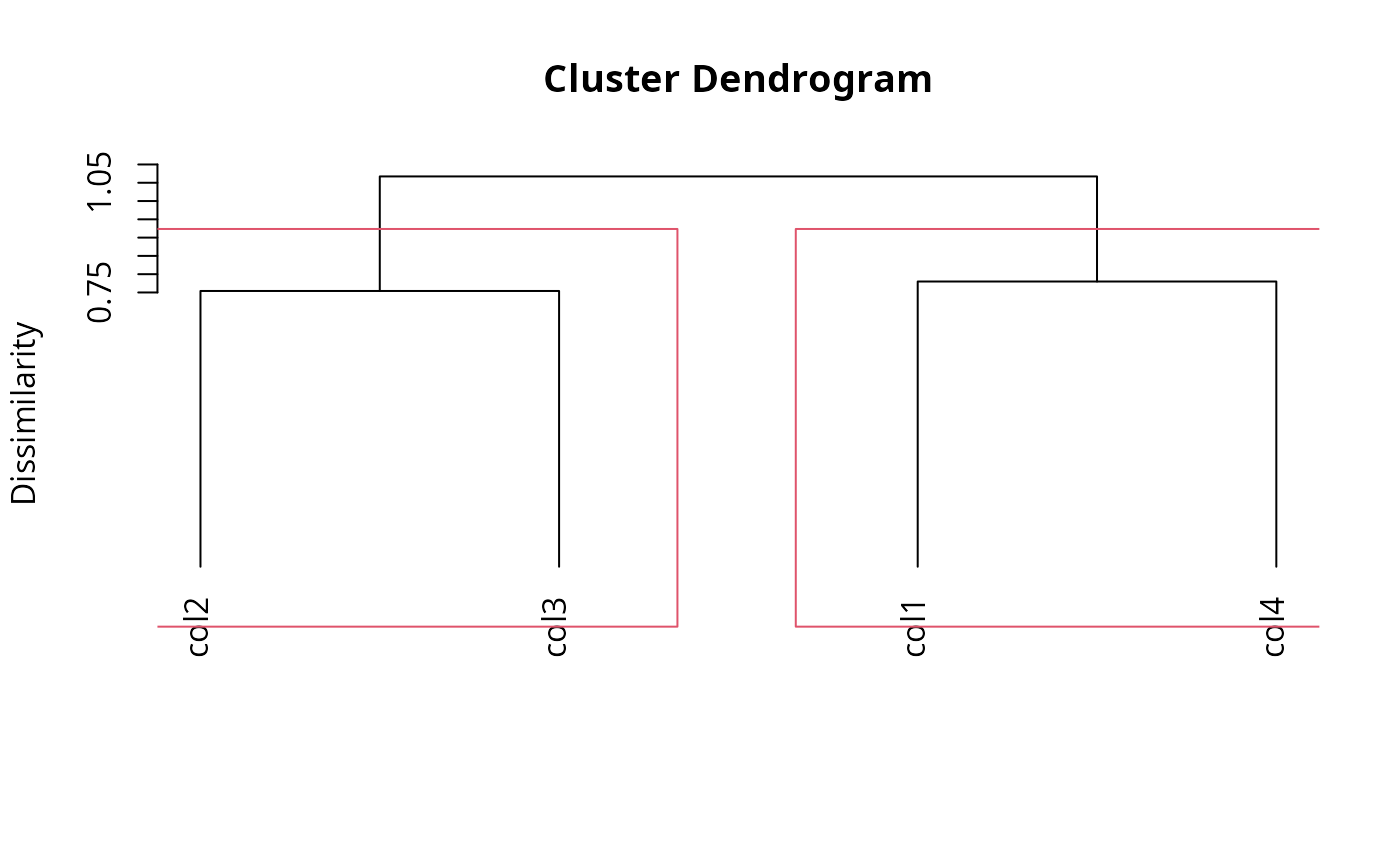
tree_mix <- build_tree(data = data, weights = "w")
plot(tree_mix)
rect.hclust(tree = tree_mix, k = 2)
 head(tree_mix$merge)
#> [,1] [,2]
#> [1,] -2 -3
#> [2,] -1 -4
#> [3,] 1 2
head(tree_mix$height)
#> [1] 0.7540818 0.7799578 1.0673062
head(tree_mix$merge)
#> [,1] [,2]
#> [1,] -2 -3
#> [2,] -1 -4
#> [3,] 1 2
head(tree_mix$height)
#> [1] 0.7540818 0.7799578 1.0673062