Table of Contents
Functional Form
Functional form is usually presented for linear models in the descriptive or explanatory modeling setting, although it’s also relevant for prediction models. Tree-based models, commonly used for prediction modeling, require no specification of functional form and automatically allow complex interactions. A downside of tree-based methods is that binary splits may not adequately capture the information contained in continuous variables.
The most common form of a linear regression model is through simple additivity of each parameter.
\[ Y = b_0 + b_1X_1 + b_2X_2 + \dots + b_pX_p + \epsilon\]
If we need to allow effect modification, where the effect of one variable depends on the values of another, then interactions terms are required (\(Y = b_0 + b_1X_1 + b_2X_2 + b_3X_1X_2 + \dots\)). Or, if nonlinearity is required, (fractional) polynomial terms may be added (\(X_1^{0.5}, X_2^2, X_3^3, \text{etc.}\)). The problem is that the functional form is almost never obvious, or even surmisable by subject matter experts ahead of time, and impractical in situations with hundreds or thousands of possible predictors. If the data size is sufficient, defaulting to restricted cubic splines for numeric variables and exploratory data analysis for interaction effects may be a good option.
When linearity in relationship between the outcome and predictors needs to be relaxed, possible methods for transforming continuous variables include:
- Dichotomization
- Why it’s used
- Simple to implement and easy to interpret.
- Where it fails
- Never recommended as it throws away too much information.
- The true relationship is almost never stepwise dichotomous.
- Why it’s used
- 3+ categories
- Why it’s used
- Simple to implement and easy to interpret.
- May be a good choice for visualizations.
- Where it fails
- Slightly better than dichotomization, but still dependent on (incorrect) cut-points and does not capture smooth relationships.
- Why it’s used
- Log, square root, inverse/exponent, Box-Cox transformations
- Why it’s used
- Simple to implement.
- May provide a mathematically convenient way to capture nonlinearity.
- Where it fails
- Harder to interpret.
- Why it’s used
- Fractional polynomials
- Why it’s used
- A flexible fit simpler than splines.
- May be justified through physical definition.
- Where it fails
- Unstable tails and tends to overfit.
- Harder to interpret.
- Why it’s used
- Smoothing splines (various choices for basis functions)
- Why it’s used
- Flexible fit and stable tails.
- Robust to many real world situations.
- Visualization using average partial effect plots may provide easy interpretation.
- Where it fails
- Not simple to implement.
- Interpretation is only through average partial effect plots.
- Why it’s used
Basic transformations
The Box-Cox procedure is a classic method used for correcting skewness of the distribution of model errors, unequal variance of model errors, and nonlinearity of the regression function. It identifies a transformation from the family of power transformations for the outcome variable. Transforming the outcome changes the variance of the outcome and the resulting errors. Transforming a predictor variable is useful for capturing nonlinearity in its relationship with the outcome.
For linear model \[ Y^{\lambda} = b_0 + b_1X_1 + \epsilon \] the Box-Cox method (Box and Cox 1964) uses the method of maximum likelihood to estimate \(\lambda\), where values of \(\lambda\) correspond to the following: \[ \begin{aligned} \lambda &= 2 \implies Y^2 \\ \lambda &= 0.5 \implies \sqrt{Y} \\ \lambda &= 0 \implies log(Y) \\ \lambda &= -0.5 \implies \frac{1}{\sqrt{Y}} \\ \lambda &= -1 \implies \frac{1}{Y} \end{aligned} \]
The natural logarithm is one of the most commonly used transformations because
- \(\frac{d}{dx}e^x = e^x\)
- \(\frac{d}{dx} ln(x) = \frac{1}{x}\)
- An exponential growth function \(Y = b_0\left( e^{b_1X_1}\right)\) can be represented as \(log(Y) = log(b_0) + b_1X_1\) after logging both sides. It converts an exponential growth to a linear growth.
- A power curve \(Y=b_0 \left( X_1^{b_1} \right)\) can be represented as \(log(Y) = log(b_0) + b_1log(X_1)\) after logging both sides. It converts a power curve into a linear function.
- The change in natural log, for small changes, is approximately the percent change.
- Log transformations spread out values close to each other and reduces the spread of values far apart.
- Log transforming Y may reduce heteroscedasticity.
- Log transforming X may efficiently handle values that spread multiple orders of magnitude.
A potential issue with log transformations is that negative values, or zero, are undefined. If your data has zeros, the square root transformation or adding a small constant before log transformation may be a possible solution.
Log transformed model terms have the following interpretations:
- Logistic models
- Log transformed predictor
- Suppose the natural logarithm was used for transformation of predictor \(X_1\) and the estimated log-odds coefficient for \(log(X_1)\) was \(\hat{\beta}_1\) with odds ratio \(e^{\hat{\beta}_1}\). We can calculate the change in odds of the outcome based on a percent change in the original units of the predictor. A \(c\%\) change in \(X_1\) is associated with a multiplicative change in \(X_1\) as \(m = \left( 1 + \frac{c}{100} \right)\).
- A \(c\%\) change in \(X_1\) multiplies the odds of the outcome by \(m^{log(e^{\hat{\beta}_1})} = e^{log(e^{\hat{\beta}_1})log(m)}\).
- Log transformed predictor
- OLS models
- Log transformed predictor
- Suppose the natural logarithm was used for transformation of predictor \(X_1\) and the estimated coefficient for \(log(X_1)\) was \(\hat{\beta}_1\). We can calculate the change in units of the outcome based on a percent change in the original units of the predictor. A \(c\%\) change in \(X_1\) is associated with a multiplicative change in \(X_1\) as \(m = \left( 1 + \frac{c}{100} \right)\).
- A \(c\%\) change in \(X_1\) changes the outcome by \(log(m) \hat{\beta}_1\) units.
- Log transformed outcome
- Suppose the natural logarithm was used for transformation of outcome \(Y\) and the estimated coefficient of \(X_1\) was \(\hat{\beta}_1\).
- A one unit increase in \(X_1\) changes the outcome by \(100\left(e^{\hat{\beta}_1} - 1\right)\%\). Or we can say the multiplicative change in the outcome was \(e^{\hat{\beta}_1}\).
- Log transformed predictor and outcome
- Suppose the natural logarithm was used for transformation of outcome \(Y\), transformation of predictor \(X_1\), and the estimated coefficient of \(log(X_1)\) was \(\hat{\beta}_1\). A \(c\%\) change in \(X_1\) is associated with a multiplicative change in \(X_1\) as \(m = \left( 1 + \frac{c}{100} \right)\).
- A \(c\%\) change in \(X_1\) changes the outcome by \(100\left( m^{\hat{\beta}_1} - 1\right)\%\). Or we can say the multiplicative change in the outcome was \(m^{\hat{\beta}_1}\).
- Log transformed predictor
When the outcome is log transformed and \(E(log(Y) | X) \sim N(\mu, \sigma^2)\), it follows that \[ \begin{aligned} \text{Mean}(Y) &= e^{\mu + \frac{\sigma^2}{2}} \\ \text{Median}(Y) &= e^{\mu} \\ \text{Var}(Y) &= (e^{\sigma^2} - 1)e^{2\mu + \sigma^2} \end{aligned} \]
where \(\hat{\mu} = e^{b_0 + b_1X_1 + \cdots + b_pX_p}\) and \(\hat{\sigma}^2\) is the MSE. Thus, when \(log(Y)\) has been used and we wish to backtransform onto the original \(Y\) scale, our naive estimate corresponds with the median, or more accurately, the geometric mean (Bland and Altman 1996; Rothery 1988). The last part following from \[ \begin{aligned} \text{Arithmetic mean}, \ AM(X) &= \frac{\sum_i^nx_i}{n} \\ \text{Geometric mean}, \ GM(X) &= \sqrt[\LARGE{n}]{\prod_i^n x_i} \\ &= e^{AM(\log(X))} \end{aligned} \]
Smoothing splines
Smoothing splines are used to model nonlinear effects of continuous covariates. Splines may be used in linear models as a linear representation of derived covariates (piecewise polynomials), or in more integrated models such as generalized additive models (GAM). GAMs were introduced by Hastie and Tibshirani (1986) and combined the properties of GLMs and (nonparametric) additive models. In contrast to using splines in a (G)LM, GAMs apply a roughness penalty to the spline coefficients which balances the goodness of fit and roughness of the spline curve. These three model types are defined as:
- Linear Model \[ \begin{aligned} y &\sim N(\mu, \sigma^2) \\ \mu &= b_0 + b_1X_1 + b_2X_2 + \dots + b_pX_p \end{aligned} \]
- Generalized Linear Model \[ \begin{aligned} y &\sim N(\mu, \sigma^2) \\ g(\mu) &= b_0 + b_1X_1 + b_2X_2 + \dots + b_pX_p \end{aligned} \]
- Generalized Additive Model \[ \begin{aligned} y &\sim N(\mu, \sigma^2) \\ g(\mu) &= f(X) \end{aligned} \]
To develop the idea of restricted cubic splines (and natural cubic splines), first consider a polynomial of degree 3 \[ Y = b_0 + b_1u_i + b_2u_i^2 + b_3u_i^3 + \epsilon \] where \(u\) us known as the basis function of \(x\). \[ U = \begin{bmatrix}1 & x_1 & x_1^2 & x_1^3 \\\ \vdots & \vdots & \vdots & \vdots \\\ 1 & x_n & x_n^2 & x_n^3\end{bmatrix} \] This simple formula leads to overfitting and non-locality (changing \(y\) at one point will cause changes in fit for data points very far away).
Next, consider a simple linear spline. For chosen knot locations \(a\), \(b\), and \(c\), the piecewise linear spline function is given by \[ y = b_0 + b_1X + b_2(X-a)_{+} + b_3(X-b)_+ + b_4(X-c)_+ \] where \[ \begin{aligned} (u)_+ = \ &u, u > 0, \\ & 0, u \leq 0 \end{aligned} \] which can be expanded to \[ \begin{aligned} y &= b_0 + b_1X, \ \text{if} \ X \leq a \\ &= b_0 + b_1X + b_2(X-a), \ \text{if} \ a < X \leq b \\ &= b_0 + b_1X + b_2(X-a) + b_3(X-b), \ \text{if} \ b < X \leq c \\ &= b_0 + b_1X + b_2(X-a) + b_3(X-b) + b_4(X-c), \ \text{if} \ c < X \end{aligned} \] The continuous piecewise linear model is constrained to connect at the knots (whereas the piecewise constant fit creates discontinuous steps). Overall linearity in \(X\) can be tested by \(H_0: b_2=b_3=b_4=0\) (Harrell 2015).
An improved method for flexible regression fits is known as restricted cubic splines (RCS). RCS doesn’t suffer from overfitting and non-locality issues seen in cubic polynomial regression and is not restricted to simple linear stepwise fits as seen in piecewise linear splines. Restricted cubic splines are built from piecewise cubic polynomials (piecewise refers to the window for each segment as defined by the knots). Natural cubic splines are essentially the same thing, but may differ in definition of basis (using B-splines?), see splines::ns (R Core Team 2021) and (Royston and Parmar 2002). RCS has continuous first derivatives, continuous second derivatives, is allowed to behave as a higher order polynomial at chosen knot points, and is required to be linear outside the boundaries of the knots. \(K\) knots results in \(K+1\) degrees of freedom. The model builder only needs to choose how many knots to use and the locations of where to place the knots.
For chosen knot locations \(t_1, \dots, t_k\), the RCS linear function is given by
\[ y = b_0 + b_1X_1 + b_2X_2 + \cdots + b_{k-1}X_{k-1} \]
where \(X_1 = X\) and for \(j = 1, \dots, k-2\)
\[X_{j+1} = (X-t_j)^3_+ - \frac{(X-t_{k-1})^3_+(t_k - t_j)}{t_k-t_{k-1}} + \frac{(X-t_{k})^3_+(t_{k-1} - t_j)}{t_k-t_{k-1}}\]
Hmisc::rcspline.eval and rms::rcs (Harrell 2021a, 2021b) divides \(b_2, \dots, b_{k-1}\) by \(\tau = (t_k - t_1)^2\) so that each basis function for \(X\) is on the same scale and to lessen difficulties in numeric optimization. This results in the following form:
\[ y = b_0 + b_1X + b_2(X-t_1)^3_+ + b_3(X-t_2)^3_+ + \cdots + b_{k+1}(X-t_k)^3_+\]
where
\[ \begin{aligned}
b_k &= \frac{b_2(t_1-t_k)t_1-t_k + b_3(t_2 - t_k) + \cdots + b_{k-1}(t_{k-2}-t_k)}{t_k - t_{k-1}} \\
b_{k+1} &= \frac{b_2(t_1-t_{k-1}) + b_3(t_2-t_{k-1}) + \cdots + b_{k-1}(t_{k-2}-t_{k-1})}{t_{k-1} - t_k}
\end{aligned} \]
Overall linearity in \(X\) can be tested by \(H_0: b_2=b_3=\cdots=b_{k-1}=0\) (Harrell 2015).
Without subject matter expertise to pre-specify knot locations at known points of nonlinearity, Harrell (2015) recommends the following default knot locations for restricted cubic splines:
| Number of knots | Quantiles for knot locations in X |
|---|---|
| 3 | .10, .5, .90 |
| 4 | .05, .35, .65, .95 |
| 5 | .05, .275, .5, .725, .95 |
| 6 | .05, .23, .41, .59, .77, .95 |
| 7 | .025, .1833, .3417, .5, .6583, .8167, .975 |
For an intuitive sense of RCS, the following figure compares piecewise cubic polynomial fits (using linear fits at the boundaries) to restricted cubic splines:
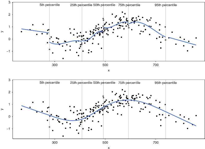 (Gauthier, Wu, and Gooley 2020)
One downside of splines is that interaction effects are nontrivial. Interactions of spline terms are known as tensor splines, and require taking all products of spline terms. rms::`%ia%` creates restricted interactions in which products involving nonlinear effects on both variables are not included in the model so that interactions are not doubly nonlinear (Harrell 2021b, 2015).