Table of Contents
Statistics Q&A
Concise questions and answers for a variety of topics. Things you should probably know off the top of your head. Most of this is summarization of texts, papers, stackexchange, or other notes. However, I’ve lost direct references for many.
Basic Stats
What is statistics?
Statistics is the scientific discipline used for designing experiments, data collection, data analysis, and interpretation of analyses for the purpose of reasoning under uncertainty.
What’s the difference between association and causation?
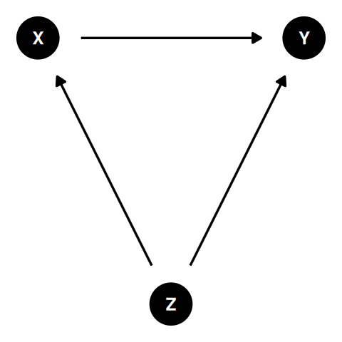
If two variables X and Y form some non-random pattern in their relationship, it can be said they are associated. However, this pattern could be the result of random chance or when there is a third variable Z which influences the previous two variables (in DAG form X←Z→Y). In addition, there may be no direction to this relationship, we can say that X is associated with Y and Y is associated with X.
If two variables X and Y have a causal association, then we can say that X influences Y when changing the state of X causes a change in the probability distribution over the values of Y. Unlike association, there is direction to this relationship. Causation doesn’t necessarily imply a deterministic relationship on an individual level, but does require a deterministic component at the population level (smoking → lung cancer).
- References
Explain the law of large numbers.
The law of large numbers shows that the sample mean converges to the population mean \(\mu\) as the sample size increases. This holds for iid observations from a distribution with finite expected value.
Borel’s law of large numbers states that if an experiment is repeated a large number of times, independently under identical conditions, then the proportion of times that any specified event occurs approximately equals the probability of the event’s occurrence on any particular trial.
Explain the central limit theorem.
The central limit theorem shows that when you sample iid observations from a distribution with finite variance the sampling distribution of the mean approaches a normal distribution.
\(\bar{x} \sim N\left( \mu, \left( \frac{\sigma}{\sqrt{n}} \right)^2 \right)\)
What is a p-value?
A p-value is the probability of how well the data we observed, or data more extreme than what we observed, fits with what was assumed under the null hypothesis and selected model. ~ \(P(data \mid \theta)\). In other words, if there was truly no difference in the population, how rare would it be to observe a sample with the calculated effect size or effect sizes even more extreme?
The p-value is a hypothetical probability derived from the test statistic’s sampling distribution. The sampling distribution is based on a hypothetical world in which the data collection and analysis method were repeated infinite times for the proposed hypothesis test. The resulting p-value is compared to the chosen type 1 error (\(\alpha\)) which is a threshold on the likelihood of the hypothetical repeated analyses to claim a significant result for a truly null comparison. If \(p \le \alpha\) we reject the null hypothesis. If \(p > \alpha\) we do not reject the null hypothesis.
The p-value is not the probability that the null hypothesis is true, and is not the probability that the results are due to chance (rather the p-value may be calculated given the assumption that the results are due to chance).
If p>0.05 should you fail to reject the null hypothesis?
Not necessarily. A large p-value simply flags the data as being not unusual if all the assumptions used to compute it (including the test hypothesis) were correct. If there were violations of those assumptions then we would expect a higher chance of incorrectly concluding to not reject the null hypothesis (false negative).
If p≤0.05 should you reject the null hypothesis?
Not necessarily. A small p-value simply flags the data as being unusual if all the assumptions used to compute it (including the test hypothesis) were correct. If there were violations of those assumptions then we would expect a higher chance of incorrectly concluding to reject the null hypothesis (false positive).
If p>0.05 does it show evidence for the null hypothesis?
No. A large p-value often indicates only that the data are incapable of discriminating among many competing hypotheses (as would be seen immediately by examining the range of the confidence interval).
If p≤0.05 does this mean the chance you’ve made a false positive conclusion is 5%?
No. If you reject the null hypothesis when it is actually true, then the chance you’ve made a false positive error is 100%. The 5% refers only to how often you would reject it, and therefore be in error, over very many uses of the test across different studies when the test hypothesis and all other assumptions used for the test are true. This statement doesn’t apply to a single test.
Statistical significance is a property of the phenomenon being studied, and thus statistical tests detect significance.
This misinterpretation is promoted when researchers state that they have or have not found “evidence of” a statistically significant effect. The effect being tested either exists or does not exist. “Statistical significance” is a dichotomous description of a p-value (that it is below the chosen cut-off) and thus is a property of a result of a study design and the statistical test; it is not a property of the effect or population being studied. In summary, significance is an attribute of the study, not of the effect.
Explain the 95% confidence interval.
Easy to understand: The confidence interval contains all values of the population statistic that we could reasonably believe to be compatible with the sample data.
Accurate: If the data collection and analysis method are valid, and repeated many times, then 95% of repeated experiments would result in a confidence interval that includes the population parameter.
The observed 95% CI has a 95% chance of containing the true effect size.
No. The frequency that an observed interval contains the true effect is either 100% if the true effect is within the interval or 0% if not. The 95% refers only to the situation if you replicated the exact same study design an infinite amount of times, then 95% of those confidence intervals would contain the true effect size if all assumptions used to compute the intervals were correct.
If two CIs overlap, the difference between two estimates or studies is not significant.
No. The 95% confidence intervals from two subgroups or studies may overlap substantially and yet the test for difference between them may still produce P < 0.05. Suppose for example, two 95% confidence intervals for means from normal populations with known variances are (1.04, 4.96) and (4.16, 19.84); these intervals overlap, yet the test of the hypothesis of no difference in effect across studies gives P = 0.03. As with p-values, comparison between groups requires statistics that directly test and estimate the differences across groups. It can, however, be noted that if the two 95% confidence intervals fail to overlap, then when using the same assumptions used to compute the confidence intervals we will find P < 0.05 for the difference; and if one of the 95% intervals contains the point estimate from the other group or study, we will find P > 0.05 for the difference.
What is type 1 error?
The probability of rejecting a true null hypothesis. AKA false positive.
\(\alpha\)
What is type 2 error?
The probability of failing to reject a false null hypothesis. AKA false negative.
\(\beta\)
When do you need to adjust for multiple comparisons?
When you test multiple hypothesis using frequentist methods, want to control for possibly increasing number of false positive results, and can allow for increased proportion of false negatives.
What is the probability of at least one false positive among multiple independent hypothesis tests?
If n independent hypothesis are tested and each of the null hypothesis are actually true, then the probability that at least one of them will be rejected is \(1 - (1 - \alpha)^n\).
For example, when \(\alpha\)=0.05 and n=20, then \(P(\geq 1 \text{ false positive})=0.64\).
The probability of not making any false rejections in a set of \(n\) tests is \((1 - \alpha)^n\).
What’s the difference between a p-value and an FDR adjusted p-value?
p-value
If the data collection and analysis method were repeated many times for a single test, we expect no more than \(\alpha\) of the hypothetical repeated analyses to claim a significant result for a truly null comparison.
False discovery rate (FDR) adjusted p-value
Among a set of independent hypothesis tests that are significant at the chosen \(\alpha\) level, we expect no more than \(\alpha\) of them to be falsely significant. For example, if \(\alpha = 0.01\), we expect that 1% of the tests with FDR adjusted p-value as small or smaller to be false positives.
To calculate an FDR adjusted p-value: 1) order all p-values from smallest to largest, 2) multiply each p-value by the total number of tests, 3) divide this value by the rank order of the p-value, 4) make sure this sequence of transformed p-values is non-decreasing by setting the preceding transformed p-value to the smaller value (repeatedly until the condition is satisfied), and 5) set transformed p-values greater than 1 to 1.
The FDR adjusted p-value and q-value are not the same thing. The FDR adjusted p-value controls the expected FDR and guarantees that the true FDR rate will be less than the specified rate on average over repeated data collection and analyses. The FDR adjusted p-value based on the BH approach is slightly more conservative than the q-value, but holds regardless of the number of tests, whereas the q-value is an asymptotic value for providing an unbiased estimate of the FDR.
Note that the FDR adjusted p-value is one way to control/define type 1 error rates under multiple hypothesis testing. The distinction between the common methods [1]:
Null True Alternative True Total Not Significant U T \(m\)-R Significant V S R Total \(m_0\) \(m-m_0\) \(m\) Where a set of \(m\) hypothesis are tested, \(m_0\) is the number of true null hypothesis, and R is the number of rejected null hypothesis.
- Per comparison error rate (PCER)
- The expected value of the number of Type 1 errors over the number of hypotheses
- \(\frac{E(V)}{m}\)
- Per-family error rate (PFER)
- The expected number of Type 1 errors in a family of hypotheses
- \(E(V)\)
- Family-wise error rate (FWER)
- The probability of at least one type 1 error
- \(P(V \geq 1)\)
- False discovery rate (FDR)
- The expected proportion of Type 1 errors among the rejected hypotheses
- \(E \left(\frac{V}{R} \mid R>0\right)P(R>0)\)
- Positive false discovery rate (pFDR)
- The rate that discoveries are false
- \(E \left(\frac{V}{R} \mid R>0\right)\)
What is power?
The power of a test to detect a correct alternative hypothesis is the pre-study probability that the test will reject the null hypothesis (e.g., the probability the p-value will not exceed a pre-specified cut-off such as 0.05). The corresponding pre-study probability of failing to reject the test hypothesis when the alternative is correct is one minus the power, also known as the Type-II or beta error rate. As with p-values and confidence intervals, this probability is defined over repetitions of the same study design and so is a frequency probability.
Stated concisely, power is the probability of correctly rejecting the null hypothesis, given that the alternative hypothesis is true.
What information is needed for power analysis and sample size calculation?
- Verify the question of interest and the variables/information needed for analysis of this question.
- Verify you are able to collect a representative sample for the question of interest.
- Check if there is previously published data for the question of interest.
- Determine the alpha level required.
- Determine the minimum relevant effect size.
- If the outcome is continuous, determine the population standard deviation. If the outcome is binary, determine the probability of the event in the control arm.
Standardized effect sizes are nice as they remove the need to specify variance. Raw effect sizes are easier to visualize and interpret.
Is it ok to calculate retrospective power?
Very rarely. Retrospective power analyses can be conducted by 4 methods:
- Using both the observed effect size and variance.
- Issues:
- Both the p-value and power are dependent upon the observed effect size and so are inversely related such that tests with high p-values tend to have low power and visa-versa. Therefore calculating power using the observed effect size and variance is simply a way of re-stating the statistical significance of the test. In addition, this method will result in an over-estimate of the true power and the point estimates are often imprecise. The estimate of the observed statistical power is not meaningful because there is no way to be sure that the effect size estimate from the study is the true parameter.
- Issues:
- Only the observed variance
- Benefits:
- Using observed variances but not observed effect sizes is helpful because it allows one to evaluate whether the sample size and alpha level were sufficient to have a good chance of detecting a biologically significant effect given the observed level of variation. You may report power over a range of effect sizes or determine the minimum effect size detectable for a given power.
- Benefits:
- Neither the observed effect size nor variance
- Issues:
- Using standardized effect sizes avoids the need to specify sampling variances, so we only use the sample size and alpha level from the study. The result will provide information to evaluate the study design, but makes it much harder to assess biological significance.
- Issues:
- Avoided completely by computing confidence intervals about the observed effect size.
- Issues:
- This method is only relevant before the results of the hypothesis test are known.
- Issues:
Since the goal is often to simply quantify the uncertainty in the findings of a study, calculating confidence intervals are more appropriate than retrospective power. If the goal is to evaluate the ability of a study to detect a biologically meaningful pattern, then retrospective power might be useful. Calculating power using pre-specified effect sizes (or calculating detectable effect size using pre-specified power) is helpful, especially if easily interpreted raw effect size measures are used. Standardized measures may be useful in more complex tests (such as tests for interaction in multi-way ANOVA) where it is hard to specify an intuitive raw measure of effect size. In these cases power analysis may be performed using conventional levels of effect size, such as those proposed by Cohen (1988). All power calculations should be accompanied by a sensitivity analysis. For power calculations that use assumed values for the effect size or variance, this means using a range of plausible values for each variable. Graphs showing how two or more variables interact with one another are particularly valuable. For power calculations that use values estimated from sample data (such as sampling variance), a confidence interval about the power estimate should be given.
References:
- Using both the observed effect size and variance.
What’s the difference between incidence and prevalence?
Prevalence refers to the number of subjects with the outcome of interest divided by the total number of subjects. It is calculated at a single moment in calendar time or based on a specific moment in time that each subject would experience.
\[\frac{\text{Number of subjects with outcome at specific time}}{\text{Total number of subjects}}\]
Period prevalence is a modification of prevalence that counts all cases which occur during a specific duration of time. It counts all outcomes of interest at the beginning time period and the cases which develop within the specified time period. You might refer to the result as a ‘1-month period prevalence’ or ‘1-year period prevalence’
\[\frac{\text{Number of subjects with outcome during time period}}{\text{Total number of subjects}}\]
Incidence refers to the number of subjects which develop the outcome of interest in a fixed time period divided by the total number of subjects at risk of developing the outcome. Subjects already with the outcome of interest are not included in the numerator or denominator. Since follow-up duration may be different between subjects, you can compute e.g. subject-months or subjects-years instead of number of subjects in the denominator.
\[\frac{\text{Number of subjects who developed outcome during time period}}{\text{Total number of subjects at risk of developing outcome}}\]
References:
What is selection bias?
Selection bias occurs when the sampled data has characteristics that are not representative of the population you wish to make make inference on. The consequence of selection bias is that the estimated association between the exposure and outcome differs from the true association among the population.
Some specific cases of this bias occur from inappropriate selection of controls in case-control studies, bias resulting from differential loss-to-follow up, incidence–prevalence bias, volunteer bias, healthy-worker bias, and nonresponse bias.
References:
What is the mean?
A measure of central tendency for a numeric variable.
\[ \bar{y} = \frac{\sum_{i=1}^{n} y_i}{n} \]
What are variance and standard deviation?
- Variance: Dispersion of a variable in squared units
- Standard deviation: Dispersion of a variable in original units. The average distance of each value from the mean.
\[ Var(y) = \frac{\sum_{i=1}^{n} (y_i - \bar{y})^2}{n-1} \]
\[ SD(y) = \sqrt{Var(y)} \]
What is the standard error?
The standard error is the standard deviation of a statistics sampling distribution.
- For single Mean: \(se = \frac{sd}{\sqrt{n}}\)
- Difference of means (equal variance): \(se = \sqrt{sd^2 \left( \frac{1}{n_1} + \frac{1}{n_2} \right)}\)
- Difference of means (unequal variance): \(se = \sqrt{\left( \frac{sd^2_1}{n_1} + \frac{sd^2_2}{n_2} \right)}\)
What is covariance?
How two variables vary linearly together in the original units. A positive value means that they move linearly in the same direction. A negative value means they move linearly in the opposite direction. A value of zero means they are not linearly related.
\[\begin{equation} \begin{aligned} Cov(X, Y) &= E[(X - \mu_{X})(Y - \mu_{Y})] \\ &= E(XY) - E(X)E(Y) \\ &= \frac{\sum_{i=1}^{n} [(x - \bar{x}) (y - \bar{y})]}{n-1} \end{aligned} \end{equation}\]
What is Pearson’s correlation coefficient?
The standardized covariance between two numeric variables: ranges from -1 to 1. A measure of strength as to how the paired values fit a line.
\[\begin{equation} \begin{aligned} \rho_{X, Y} &= \frac{Cov(X, Y)}{\sigma_X \sigma_Y} \\ &= \frac{E[(X - \mu_{X})(Y - \mu_{Y})]}{\sigma_X \sigma_Y} \\ &= \frac{E(XY) - E(X)E(Y)}{\sqrt{E(X^2)-(E(X))^2}\sqrt{E(Y^2)-(E(Y))^2}} \\ &= \frac{\sum_{i=1}^{n}(x_i - \bar{x})(y_i - \bar{y})}{\sqrt{\sum_{i=1}^{n} (x_i - \bar{x})^2}\sqrt{\sum_{i=1}^{n} (y_i - \bar{y})^2}} \end{aligned} \end{equation}\]
Paradoxes, Phenomena, and Fallacies
What is Simpson’s paradox?
This paradox was described in detail by Edward Simpson in 1951. It occurs when the relationship between two categorical variables reverses (or is diminished or enhanced) when you condition on a third categorical variable. Consider the situation where, as a whole, the control group was more likely to get sick than those who took a drug \((\frac{13}{60} = 0.22 > \frac{11}{60} = 0.18)\). However, within each gender, the control group had a smaller chance of getting sick than those who took the drug: \((\frac{1}{20} = 0.05 < \frac{3}{40} = 0.07 \text{ and } \frac{12}{40} = 0.3 < \frac{8}{20} = 0.4)\). This reversal in relative frequency is because of the mathematical property that if \(\frac{A}{B} > \frac{a}{b} \text{ and } \frac{C}{D} > \frac{c}{d}\) does not imply that \(\frac{A + C}{B + D} > \frac{a + c}{b + d}\). In this case \(\frac{3}{40} > \frac{1}{20}\) and \(\frac{8}{20} > \frac{12}{40}\) but \(\frac{3 + 8}{40 + 20} < \frac{1 + 12}{20 + 40}\).
Both the control and drug groups had 60 people total. However, the control group had 40 men while the drug group had 20 men, and men were overall more likely to get sick \((\frac{20}{60} = 0.33 > \frac{4}{60} = 0.07)\). Looking at the aggregated data hides this fact and results in Simpson’s paradox.
control
drug
sick
healthy
total
sick
healthy
total
female
1
19
20
3
37
40
male
12
28
40
8
12
20
total
13
47
60
11
49
60
You might think this means the conditional analysis is always the correct choice, however, the only way to formally decide is to draw the relevant causal networks, decide on which variables are confounding, and make those assumptions known when reporting the results. Choosing the correct way to analyze data is not based on naively conditioning on every variable measured, but rather is extracted from the context of the question, the data generating process, and design of experiment.
References:
What is Lord’s paradox?
This paradox was described in detail by Frederic Lord in 1967. It occurs when the relationship between two variables (one categorical and one continuous) reverses (or is diminished or enhanced) when you condition on a third continuous variable. The usual example for the third variable is a baseline measurement, while the outcome (response) is the final measurement. There are two options for analysis
- An unconditioned test on the change score
- A conditioned test on the final outcome.
A t-test on the change score, \(y - x2\), provides a summary for the total effect (direct effect of x1 plus indirect effects through all others paths), while an ANCOVA with baseline as a covariate provides the direct effect of x1.
In a pre-post design, if differences between treatment groups at baseline are expected to be zero (such as in a RCT), then a baseline adjusted model and change score model are expected to give the same result. If differences between the two treatment groups are expected, then the two methods are expected to give different results. Thus, the researcher needs to choose the causal mediation effect of interest in order to have a meaningful interpretation.
References:
What is Suppression?
Suppression occurs when the relationship between two continuous variables reverses (or is diminished or enhanced) when you condition on a third continuous variable. The general case is observed when an explanatory variable that is unrelated to the response variable increases the fit of a model. Suppose a model has continuous response y and continuous explanatory x1 and x2. If \(corr(y, x1) = 0\) and \(corr(y, x2) > 0\) and \(corr(x1, x2) > 0\) then including x1 can suppress the part of x2 that is uncorrelated with y. The coefficient for x2 can increase, \(R^2\) can increase, and the coefficient for x1 will be less than zero. In general, suppression is seen when controlling for a ‘third’ variable that is termed a confounder (although this confounder can only be interpreted based on a causal diagram in context of the question).
References:
What is Berkson’s paradox?
In 1946, Joseph Berkson, a biostatistician at the Mayo Clinic, noticed that even if two diseases have no relation to each other in the general population, they can be associated among hospital patients. This can result from a situation where neither of the two diseases by themselves cause hospitalization, but together they do. So conditioning on hospitalization created a spurious association between the two diseases. Determining this effect is hard, and it’s important to create causal diagrams to illustrate the potential confounding paths. This often arises from convenience samples or other sampling bias.
What is Will Roger’s phenomenon?
This phenomenon is attributed (maybe incorrectly) to comedian Will Rogers with the following quote:
“When the Okies left Oklahoma and moved to California, they raised the average intelligence level in both states.”
This is more generally referred to as stage migration. For example, improved detection of illness leads to an increased number of unhealthy people which can result in a increase in life span for both groups even if no improvement in treatment is seen. This is a potential explanation for the increase in cancer survival times. In summary, you may wrongly attribute to treatment effects and should be conditioning on diagnostic criteria.
What is regression to the mean?
In 1885, Francis Galton published a paper on the height of parents and their children. He found that parents on the extreme ends of the height spectrum tend to have children whose height is closer to the average. This effect causes issues when selection for measurement is based on some criterion (above or below a certain value) from an initial measure. Consider the situation where you measure blood pressure for 1000 patients and 285 had DBP values greater than 95mmHg. Instead of following up with all 1000 patients, you only called back the 285 and find that their mean DBP value has decreased. In this situation you would not be able to separate the effect of a drug or other intervention from regression to the mean. To see the effect of an intervention, you would need to randomly assign half of the 285 to a control group and half to a treatment group. Then both groups would have the same regression to the mean improvement and any differences could be attributed to the treatment.
References:
What is Stein’s paradox?
This paradox was described in detail by Charles Stein in 1955 [1] and later refined with Willard James in 1961 [2]. Suppose \(X_1, X_2, ..., X_k\) are independently normal random variables such that \(X_i \sim N(\theta, I)\) where \(\theta = \theta_1, \theta_2, ..., \theta_k\) and \(I\) is the \(k \times k\) identity matrix. It turns out that the best estimator for \(\hat{\theta}_i\) is not \(\bar{x}_i\), but rather \(\hat{\theta}^\prime_i = \bar{\bar{x}} + c(\bar{x}_i - \bar{\bar{x}})\) where \(\bar{\bar{x}}\) is the grand mean and \(c = 1 - \frac{(k-3)\sigma^2}{\sum(\bar{x}_i - \bar{\bar{x}})^2}\) is a constant. It’s possible for \(c\) to be negative, thus should be replaced with 0 for these cases to produce better estimations.
This estimator is not intuitive as it requires combining information from independent populations to produce a more optimal estimator of each population’s mean. The James-Stein estimator is similar to that of Bayes’s equation and is often referred to as empirical Bayes estimator (closer in likeness as \(k\) increases). In the Bayes perspective, the independent samples are joined through the common prior for \(\theta\) and the resulting pooled estimate is similar to James-Stein.
As described in [3], shrinkage is only possible when \(K \ge 3\). The intuition for this can be seen using linear regression. When there are only one or two observations, the linear regression line must pass through those exact points. When there are three or more observations, the regression line represents the James-Stein estimator.
Quoting from Efron and Morris [4]:
What do these equations mean in terms of the behavior of the estimator? In effect the James-Stein procedure makes a preliminary guess that all the unobservable means are near the grand mean (\(\bar{\bar{x}}\)). If the data support that guess in the sense that the sample means are themselves not too far from \(\bar{\bar{x}}\), then the estimates are all shrunk further toward the grand mean. If the guess is contradicted, then not much shrinking is done. These adjustments to the shrinking factor are accomplished through the effect the distribution of means around the grand mean has on the equation that determines c. The number of means being estimated also influences the shrinking factor, through the term (k - 3) appearing in this same equation. If there are many means, the equation allows the shrinking to be more drastic, since it is then less likely that variations observed represent mere random fluctuations. …
The James-Stein estimator does substantially better than the sample means only if the true means lie near each other, so that the initial guess involved in the technique is confirmed. What is surprising is that the estimator does at least marginally better no matter what the true means are.
- [1] https://projecteuclid.org/ebook/Download?urlid=bsmsp%2F1200501656&isFullBook=False
- [2] https://projecteuclid.org/ebook/Download?urlid=bsmsp%2F1200512173&isFullBook=False
- [3] https://projecteuclid.org/journals/statistical-science/volume-5/issue-1/The-1988-Neyman-Memorial-Lecture--A-Galtonian-Perspective-on/10.1214/ss/1177012274.full
- [4] https://doi.org/10.1038/scientificamerican0577-119
What is the Jeffreys-Lindley paradox?
This paradox was discussed by Harold Jeffreys in 1939 [1] and later by Dennis Lindley in 1957 [2]. It centers around the opposition between the frequentist and Bayesian schools of inference in terms of decision rules. This can be seen when the decision to reject or not reject the null hypothesis using a t-test may lead to different conclusions from the comparable Bayesian procedure using Bayes factors (which are a measure of evidence brought by the data in favor of the null hypothesis relative to the alternative) [3]. David Colquhoun [4] reframes the paradox using false positive risk (FPR). FPR is the probability that a result which is “significant” at a specified p-value is a false positive result. Thus, if p=0.05, the FPR actually increases as the sample size increases. In other words, p=0.05 provides strong evidence for the null hypothesis at large sample sizes. So, in situations with very high power to detect an effect, p-values close to traditional cut-offs don’t necessarily provide the correct decision?
What is the absence of evidence fallacy?
The absence of evidence fallacy (argument from ignorance, appeal to ignorance) is a formal logical fallacy. It is explained in the statistical perspective by Douglas Altman and Martin Bland [1] in their note, “Absence of evidence is not evidence of absence”. In other words, failing to reject the null hypothesis for a test of difference does not imply evidence for no difference. All that has been shown is an absence of evidence of a difference, nothing more.
What is the ecological fallacy?
The ecological fallacy occurs when statistical analyses are made on aggregated group-level data, but interpretations are applied to the individuals who made up those groups. The erroneous results are often due to uncontrolled confounding? Ecological fallacies are often seen in misinterpretations of meta-analysis.
What is the prosecutor’s fallacy?
This fallacy also goes by the names base-rate fallacy, inverse fallacy, or transposed conditional error. Using legal terms, it’s making the error that \[P(\text{innocent} \mid \text{evidence}) = P(\text{evidence} \mid \text{innocent}),\] when in reality \[P(\text{innocent} \mid \text{evidence}) = \frac{P(\text{innocent})P(\text{evidence} \mid \text{innocent})}{P(\text{evidence})}\] Or, in general terms, making the error that \[P(\text{Data} \mid H_0) = P(H_0 \mid \text{Data}).\]
The simplest example can be seen as \(P(\text{Doctor} \mid \text{Surgeon}) = 1\), however \(P(\text{Surgeon} \mid \text{Doctor})<1\).
Errors may arise in the medical setting when the prevalence of a disease is ignored while interpreting diagnostic results. Suppose the false positive rate of a medical test is 1/100 (1 chance in a 100 that the test says positive in cases that are actually negative) and the prevalence in the population is 1/1000. This means that with no other evidence to predispose you to having the disease, you have 10:1 odds that the test was incorrect.
As another example, suppose the prevalence of a disease (D) is 1/1000. The sensitivity of a test (probability the test is positive given the person has the disease) is 0.8 and the specificity (probability the test is negative given the person does not have the disease (H)) is 0.8. Assuming a person was tested at random with no other evidence suggesting disease:
\[\begin{aligned} P(D \mid +) &= \frac{P(+ \mid D)P(D)}{P(+)} \\ & = \frac{P(+ \mid D)P(D)}{P(+ \mid D)P(D) + P(+ \mid H)P(H)} \\ & = \frac{P(+ \mid D)P(D)}{P(+ \mid D)P(D) + (1 - P(- \mid H))P(H)} \\ & = \frac{0.8 \times 0.001}{0.8 \times 0.001 + 0.2 \times 0.999} \\ & = 0.004 \end{aligned}\]
So our knowledge has increased from the baseline probability of disease as 0.001 to the new probability of disease as 0.004.
What is the gambler’s fallacy?
The gamblers fallacy and hot hand fallacy are the mistaken belief that prior outcomes from a series of random events affect the probability of a future outcome. The gambler’s fallacy is believing that past outcomes make opposite outcomes more likely (e.g., “red is due” after many blacks). The hot hand fallacy is believing streaks will continue.
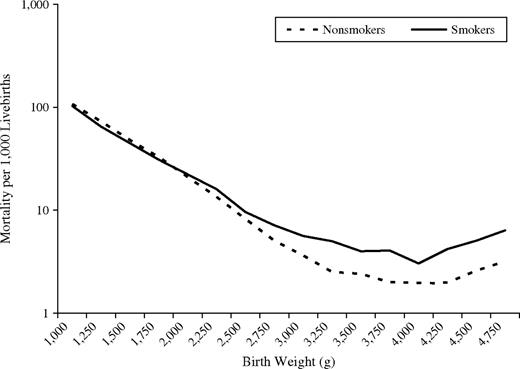
What is the low birth weight paradox?
Birth weight is a predictor of infant mortality. For this reason, and because birth weight data are readily available, investigators have frequently conditioned on birth weight when evaluating the effect of infant mortality. This often produces a crossover of the birth weight specific mortality curves. LBW infants in groups with a high prevalence of LBW have a lower mortality rate than LBW infants in groups with a low prevalence of LBW, whereas the opposite is true for normal-weight infants. This phenomenon is known as the “birth weight paradox”. Miguel Hernan et al. [1] used causal diagrams to show that this apparent paradox can be conceptualized as selection bias due to stratification on a variable (birth weight) that is affected by the exposure of interest (smoking) and that shares common causes with the outcome (infant mortality) (see also, collider bias).
What is the table 2 fallacy?
The table 2 fallacy was highlighted by Daniel Westreich and Sander Greenland [1].
It’s common in medical studies for table 1 to be a table of demographic, social, and clinical characteristics of the study groups, often categorized by levels of exposure (treatment). Table 2 is commonly a table of multivariable regression results. The multivariable model contains effect estimates for both the primary estimate of interest (exposure) and for secondary risk factors or confounders. By presenting adjusted effect estimates for secondary risk factors alongside the adjusted effect estimate for the primary exposure, Table 2 suggests implicitly that all of these estimates can be interpreted similarly, if not identically. This is often not the case. They can only be interpreted after defining the causal diagram (DAG) and if variables may summarize the primary effect, secondary effect, total effect, direct effect, and other factors in effect interpretability.
- Primary effect: The causal effect of an exposure of primary interest.
- Secondary effect: The causal effect of a covariate not of primary interest in the initial adjustment model (e.g., a confounder or effect-measure modifier).
- Total effect: The net of all associations of a variable through all causal pathways to the outcome.
- Direct effect: An association after blocking or controlling some of those pathways.
What is the Hauck-Donner effect?
The Hauck-Donner effect occurs when the log-likelihood surface is non-quadratic (such as when the sampling distribution of a parameter is not normal) and extremely large parameter estimates near the parameter space boundary are given as a result. Hauck and Donner (1977) [1] showed that the Wald test statistic does not monotonically increase as the distance between the parameter estimate and null value increases. This results in the Wald test having low power leading to nonsignificance of a potentially truly large effect.
This effect is usually framed in the context of logistic regression, but can occur in any GLM. The likelihood ratio test may be used instead of the Wald test since it only assumes a weaker asymptotic assumption that the LR statistic is proportional to a \(\chi^2_r\) distribution.
What is Freedman’s paradox?
Freedman’s paradox is based on an observation by David Freedman in 1983 [1] on how variable selection can lead to erroneous significance. For example, if a regression model is fit with many parameters then refit again on only the parameters that were significant, then the overall F-test will be incorrectly inflated.
This issue is representative of the overall issue with traditional stepwise model selection. Confidence intervals and p-values for parameter estimates are too small and the illusion of confirmatory results for model structure is promoted.
Other methods and ideas to avoid.
Commonly used methods and ideas that are statistically unsound, suboptimal, or just unnecessary for most cases. Many of these items were from Stephen Senn, Frank Harrell, https://discourse.datamethods.org/t/reference-collection-to-push-back-against-common-statistical-myths/1787, and https://ard.bmj.com/content/74/2/323.
- Do not dichotomize ordered/continuous variables.
- Dichotomizing continuous variables results in loss of information and assumes the effect on the response is a step function which only changes at the cut-point.
- https://doi.org/10.3174/ajnr.A2425
- https://doi.org/10.1002/sim.2331
- https://doi.org/10.1186/s12874-019-0667-2
- https://doi.org/10.1136/bmj.332.7549.1080
- https://doi.org/10.1093/jnci/86.11.829
- Do not use change from baseline to measure difference.
- In a baseline adjusted model, if the slope for the baseline covariate is equal to one, then the model is identical to the change score analysis. If the slope for the baseline covariate is zero, then the model is identical to ignoring the baseline value.
- Some argue that baseline adjusted models should not be used in observational data (where an exposure could be present before the baseline score was measured). See Lord’s paradox for more information.
- https://doi.org/10.1002/sim.4780111304
- https://doi.org/10.1136/bmj.323.7321.1123
- https://doi.org/10.1186/1745-6215-12-264
- https://www.fharrell.com/post/errmed/#change
- https://doi.org/10.1161/strokeaha.121.034859
- https://doi.org/10.1093/aje/kwi187
- https://content.sph.harvard.edu/fitzmaur/ala2e/
- page 126
- Do not use responder analysis.
- Do not use minimization.
- Do not use propensity scores.
- Matching is probably the worst offender here, but other flavors are unnecessary as well. Senn writes, “I like to start by comparing completely randomised and matched pair designs. In both cases the PS is 1/2. However to analyse the latter as if it were the former is regarded as an elementary error. However the point estimate is the same so what’s the problem? The problem is the standard error is different. Much confusion in discussing analysis and design arises from assuming the point estimate is the goal.”, … “What matters is whether something is predictive of outcome not of assignment.”
- https://doi.org/10.1002/sim.3133
- https://doi.org/10.1016/j.jacc.2016.10.060
- https://doi.org/10.1017/pan.2019.11
- https://www.youtube.com/watch?v=rBv39pK1iEs
- Do not use split plot analysis of repeated measures.
- Do not use sigma-divided measures.
- Examples using Cohen’s d
- John Myles White writes, “Also this is a good time for my regular reminder that Cohen’s d is only useful for power analysis. If a medical treatment lets me live one year longer, increasing the population-level variation in lifespans doesn’t decrease the value of that year for me in any way.”
- Andrew Vickers writes, “if my boss gives me a $1000 pay rise, whether I should be pleased or not depends on the standard deviation of salaries at my hospital, right?” (But we would be interested in the standard deviation of pay raises.)
- https://doi.org/10.1198/sbr.2010.10024
- Examples using Cohen’s d
- Do not report number needed to treat (NNT).
- Do not use two-stage analysis of cross-over designs.
- Do not adjust for simple carry-over.
- Do not use type III or Type I sums of squares.
- No one wants sequential sums of squares (Type I).
- Type III is either no different from the Type II and hence redundant or it is, because it adjusts an unbalanced main effect for an interaction. See chapter 14 of http://senns.uk/SIDD.html.
- Do not ignore the difference between blocks and treatments.
- Do not use global tests of significance.
- A test that assumes all levels are equal is rarely of interest. Instead, just estimate and show the specific contrasts between levels using appropriate confidence intervals.
- Do not attach a p-value to a descriptive summary.
- Descriptive summaries of a sample do not require information about statistical significance or p-values. Only when inference is made on the representative population is statistical significance relevant.
- Do not ignore covariates in a randomized controlled trial (RCT).
- Variable selection
- Do not use stepwise
- Do not use univariable screening
- Do not blindly use the word “normality” without a sentence or two that fully describes the context of the problem.
- I’ve never seen a client who understands this concept and regularly see other statisticians reinforce their misconceptions…
- In regression modeling, there isn’t concern about any variable being normal. However, the least important assumption of regression modeling does call for normality of the errors (residuals).
- Hypothesis tests for normality exist, however statisticians do not use them. Statisticians use diagnostic plots, spend a moment or two to consider any issues they might suggest, and then ignore these issues and proceed with the analysis :)
- https://doi.org/10.1186/1471-2288-12-81
- https://doi.org/10.1007/s00362-009-0224-x
- https://doi.org/10.7275/55hn-wk47
- Do not use significance testing in pilot studies.
- The purpose of pilot studies is to identify issues in all aspects of the study ranging from recruitment to data management and analysis. It isn’t concerned with making inference on population effects.
- https://doi.org/10.1136/bmj.i5239
- https://doi.org/10.1111/j.1752-8062.2011.00347.x
- Do not say the Wilcoxon test is about the median.
- Inferring anything about the median is only possible if the variables are sampled from population distributions which differ only in location, not shape or scale (which is unlikely).
- The Wilcoxon test is actually about the rank sums. Both variables can have the same 25th and 50th percentiles, yet if one has a larger 75th percentile then that may support the claim that distribution has a larger rank sum.
- https://doi.org/10.1080/00031305.2017.1305291
- Multiplicity adjustments are not necessary in exploratory studies.
- The goal of exploratory studies are to make sure we do not miss out on some potentially new and interesting finding. After observing this new finding, additional studies will need to take place to verify the results. Thus, we are not worried about making type I errors (false positives), but are worried about making type II errors (false negatives). By definition, adjusting for multiplicity increases the probability of making a type II errors to control the probability of making a type I error. Therefore multiplicity adjustments are not necessary for this study. (some caveats apply…)
- https://doi.org/10.1016/s0895-4356(00)00314-0
- https://doi.org/10.1016/j.athoracsur.2015.11.024
- https://doi.org/10.1097/00001648-199001000-00010
- https://doi.org/10.1111/brv.12315
- https://doi.org/10.1136/bmj.316.7139.1236
- https://doi.org/10.1016/j.actpsy.2014.02.001
- https://doi.org/10.1111/bju.14640
- https://doi.org/10.1186/1471-2288-2-8
- Do not use ROC optimal cutpoints.
- The sample size is often not even large enough for an accurate estimate of the population prevalence. If so, how would the data contain the information to choose the optimal cutpoint from all competing possibilities?
- ROC curves are based on sensitivity, \(P(\text{test positive} \mid \text{actual positive})\), and specificity, \(P(\text{test negative} \mid \text{actual negative})\). This means we condition on what is unknown to estimate what is known. How is this backwards reasoning relevant for individual predictions?
- ROC optimal cutpoints assume that sensitivity and specificity are constant for any given observation. However, just as the likelihood of one outcome varies from observation to observation, and is dependent upon selected predictor variables, sensitivity and specificity also vary from observation to observation and are dependent on covariates. For example, sensitivity increases along with any covariate related to outcome likelihood.
- https://doi.org/10.1002/pst.331
- https://doi.org/10.1002/sim.1611
- https://www.fharrell.com/post/backwards-probs/
- Do not use Yates’ continuity correction.
- Pearson’s asymptotic \(\chi^2\) test with Yates’ continuity correction is often the default statistic calculated in many software packages. However, Yates’ continuity correction is too conservative, similar to Fisher’s exact test.
- https://doi.org/10.1002/sim.4780090403
- https://doi.org/10.1002/sim.3531
- Do not dichotomize ordered/continuous variables.
Models
Theory
What is ordinary least squares (OLS)?
- Ordinary Least Squares (OLS) is an estimation method that corresponds to minimizing the sum of square differences between the observed and predicted values (SSE).
- The closed form solution is \(\hat{\beta} = (X^TX)^{-1} X^T Y\).
- Under the assumption that the linear model residuals are normally distributed, OLS and MLE estimators are equivalent.
- The Gauss-Markov theorem shows that the OLS estimates are the Best Linear Unbiased Estimators (BLUE) (minimum variance and unbiased) when the OLS model assumptions are satisfied (Errors have mean zero, uncorrelated, and homoscedastic. Normality of errors is not required.).
What is maximum likelihood estimation (MLE)?
- Maximum Likelihood Estimation (MLE) is an estimation method that corresponds to maximizing the likelihood function.
- The MLE estimates of the model coefficients are found through an iterative algorithm:
- Specify the statistical process (linear model) that relates the response to the predictors.
- Choose starting values for the coefficients
- Find the residual and likelihood score
- Propose new coefficient values that will improve the likelihood.
- Repeat until there is no improvement in the likelihood
- The cost function for MLE becomes minimization of the negative log-likelihood (NLL).
- The expectation maximization (EM) algorithm is a common MLE estimation method.
- Under the assumption that the linear model residuals are normally distributed, OLS and MLE estimators are equivalent.
What is Bayesian inference?
Bayesian inference can be thought of in the following three steps
- Creating the full probability model
- A joint probability model for all observable and unobservable quantities in a problem.
- Conditioning on observed data
- Calculate the posterior distribution (the conditional probability distribution of the unobserved quantities of interest, given the observed data)
- Evaluating the fit of the model and the implications of the posterior distribution.
- How well does the model fit the data?
- Are the conclusions reasonable?
- How sensitive are the results to the assumptions made in step 1?
The posterior distribution is formed using the combination of the likelihood and prior models:
- Posterior density
- \(p(\theta \mid D) = \frac{p(D \mid \theta)p(\theta)}{p(D)}\)
- Unnormalized posterior density
- \(\text{Posterior} \propto \text{Likelihood} \times \text{Prior}\)
- \(p(\theta \mid D) \propto L(\theta \mid D) p(\theta)\)
Above describes “full” Bayesian inference, where the distinction between various methods are defined as:
- MLE (maximum likelihood estimation)
- \(p(y \mid x;\theta)\), where \(\hat{\theta}_{MLE} = \text{argmax}_{\theta} p(D;\theta)\)
- Used for frequentist inference since it provides point-wise estimates of the model parameters.
- CIs and p-values are based on the idea of repeated sampling.
- MAP (maximum a posteriori)
- \(p(y \mid x,\theta)\), where \(\hat{\theta}_{MAP} = \text{argmax}_{\theta} p(\theta \mid D) \propto L(\theta \mid D)p(\theta)\)
- Partial? Bayesian inference since it only summarizes the posterior mode.
- Similar to MLE, but incorporates the prior distribution, thus creating a regularized maximum likelihood estimate.
- Full Bayesian inference
- \(p(y \mid x,D) = \int_{\theta}p(y \mid \theta, x, D)p(\theta \mid D)d\theta\)
- The full posterior distribution is used for inference.
- Conjugate prior relationships
- Creating the full probability model
What are common algorithms for optimization?
Most regression methods (e.g. non-OLS) do not have closed form (analytical) solutions for minimizing loss functions or maximization of likelihood functions (ideally convex, continuous, and differentiable functions). Various iterative algorithms are used to balance the ease of implementation, speed of convergence, numeric stability, and ability to find global maxima/minima from competing local points or singularities.
- First order (based on information from the first derivative)
- Gradient descent is a first order (derivative) method. There are many different forms of gradient descent algorithms. These different algorithms usually define new ways to estimate/modify the learning rate, add additional hyperparameters (that often need tuning…), or find minima using different sets of model parameters or subsets of the data to reduce complexity.
- It’s nice because it moves in the direction of highest improvement and will stop when it gets to a local optimum.
- Problems arise because the learning rate can be very small leading to long run-times. If the learning rate is too large, it may diverge out of control.
- Gradient descent is a first order (derivative) method. There are many different forms of gradient descent algorithms. These different algorithms usually define new ways to estimate/modify the learning rate, add additional hyperparameters (that often need tuning…), or find minima using different sets of model parameters or subsets of the data to reduce complexity.
- Second order (based on information from the second derivative)
- Newton’s method uses the first order derivative (gradient) and second order derivative (Hessian matrix) to approximate the objective function with a quadratic function. There are many different optimization algorithms that use Newton’s method.
- It’s nice because its speed of convergence is quadratic (very fast).
- Problems arise in high-dimensional models where modifications are needed to better handle saddle points. It is computationally expensive.
- See Newton-Raphson in logistic regression and L-BFGS
- Newton’s method uses the first order derivative (gradient) and second order derivative (Hessian matrix) to approximate the objective function with a quadratic function. There are many different optimization algorithms that use Newton’s method.
- Expectation Maximization
- EM iteration alternates between performing an expectation (E) step, which creates a function for the expectation of the log-likelihood evaluated using the current estimate for the parameters, and a maximization (M) step, which computes parameters maximizing the expected log-likelihood found on the E step. These parameter-estimates are then used to determine the distribution of the latent variables in the next E step.
- The MLE of a parameter can be found even in incomplete data problems (missing data, censored data, latent data).
- First order (based on information from the first derivative)
What are loss/cost/objective functions?
- Loss refers to the function defining goodness of fit applied to a single observation. For example, \(\text{loss function} = L(x_i, y_i)\). The regularization term may or may not be included?
- Cost refers to the function defining goodness of fit applied to the entire sample, and summarized as the average loss. For example, \(\text{cost function} = \frac{1}{n} \sum_{i=1}^{n}L(x_i, y_i)\). The regularization term may or may not be included?
- The objective function generally refers to the cost function including the regularization term if needed.
There are many different loss/cost/objective functions:
- Binary outcomes
- Log loss (Cross-entropy loss)
- \(L(y, p) = -[y \text{log}(p)+(1-y)\text{log}(1-p)]\), where \(y \in \{0,1\}\) and \(p=P(y=1)\).
- \(L(y, f(x)) = log(1 + e^{-yf(x)})\)
- Used in logistic regression
- Outputs well-calibrated probabilities
- Hinge loss
- Used in standard SVM models
- Exponential loss
- Adaboost loss
- Gini index
- 0-1 loss
- Log loss (Cross-entropy loss)
- Continuous outcomes
- Squared error loss
- \(L(y, f(x)) = (y - f(x))^2\)
- The loss function for OLS.
- Cost function is the mean squared error loss, AKA quadratic loss.
- Used for estimating the mean outcome, \(f(x) = E(Y \mid X=x)\).
- Advantages: Differentiable everywhere.
- Disadvantages: Sensitive to outliers.
- Absolute error loss
- \(L(y, f(x)) = |y - f(x)|\)
- Cost function is the mean absolute loss.
- Used for estimating the median outcome, \(f(x) = \text{median}(Y \mid X=x)\).
- Advantages: Not as sensitive as squared error loss.
- Disadvantages: Not differentiable at zero.
- Huber loss
\[\begin{equation}
L(y, f(x)) =
\begin{cases}
(y - f(x))^2 & \text{for } |y - f(x)| \leq \delta \\
2\delta |y - f(x)| - \delta^2 & \text{otherwise}
\end{cases}
\end{equation}\]
- Behaves like squared error loss when the loss is small and absolute error loss when the loss is large.
- Squared error loss
What is the likelihood function?
The Likelihood is a measure of the extent to which a sample provides support for each possible value of a parameter in a parametric model.
Given a probability density function \(f(x \mid \theta) = (\theta + 1)x^{\theta},\) the likelihood, \(L(\theta \mid x)\), is defined as \(L(\theta \mid x) = \prod_{i = 1}^{N}(\theta + 1)x_{i}^{\theta},\) and the corresponding log-likelihood, \(\Lambda(\theta \mid x)\), is defined as \(\Lambda(\theta \mid x) = \sum_{i = 1}^{N} \text{log}(\theta + 1) + \theta \text{log}(x_{i}).\)
If you want the maximum likelihood estimator (MLE), you need to find the maximum of the log-likelihood function: \(0 = \frac{\partial\Lambda(\theta \mid x)}{\partial\theta} = \sum_{i = 1}^{N} \frac{1}{\theta + 1} + \text{log}(x_{i}) = \frac{N}{\theta + 1} + \sum_{i = 1}^{N}\text{log}(x_{i})\)
What is the difference between a linear and nonlinear model?
A model is linear (or nonlinear) in its parameters. For example, \(y = \beta x^2 + \epsilon\) is linear in \(\beta\) but not in \(x\), while \(y = exp(\beta) x + \epsilon\) is nonlinear in \(\beta\) but linear in \(x\).
What is the difference between linear and generalized linear models?
- Linear model:
- Y, conditional on X, is normally distributed with a mean of the predicted values and some variance.
- \(Y \mid X \sim N(\beta X, \sigma^2)\)
- The error term \(\epsilon \sim N(0, \sigma^2)\)
- \(E(Y \mid X) = \beta X\)
- Fit with OLS
- Generalized linear model:
- Allows us to fit response variables that are from any exponential family (conditioning on the predictors).
- \(E(Y \mid X) = g^{-1}(\beta X)\)
- \(g(E(Y \mid X)) = \beta X\)
- \(g\) is the link function. The link function determines how the expected value of the response relates to the linear predictor.
- It also requires a variance function to determine how \(Var(Y)\) depends on the mean. \(Var(Y) = V(E(Y)).\)
- Fit with MLE
- Linear model:
What is the bias-variance tradeoff?
- Variance refers to the amount the predictions (i.e. the model) would change if the model was built using a different dataset.
- Bias refers to the error that is introduced by approximating a real life problem. The average error of a prediction.
- Noise is the inherent variability in the data.
Models that have high bias tend to have low variance. For example, simple linear regression. Models that have low bias tend to have high variance. For example, complex, flexible models. We want a model that is complex enough to capture the true relationship between the explanatory variables and the response variable, but not overly complex such that it finds patterns that don’t really exist.
You’ll commonly see the following relationship described for bias-variance decomposition. Given \(y=f(X)+\epsilon\) is the true data generating function and \(h(x) = wx+e\) is the sample fit to minimize squared error loss, we find that
\[\begin{equation} \begin{aligned} E\left[(y - h(x))^2\right] &= E\left[(h(x) - \bar{h}(x))^2\right] + (h(x) - f(x))^2 + E\left[(y - f(x))^2\right] \\ &= E\left[(h(x) - \bar{h}(x))^2\right] + (h(x) - f(x))^2 + Var(\epsilon) \\ &= \text{Variance + Bias}^2 \text{+ Noise} \\ &= \text{MSE}(h(x)) + \sigma^2 \\ &= \text{Expected prediction error} \\ &\approx CV(h(x)) \end{aligned} \end{equation}\]
Possible solutions for
- High variance
- More data
- Reduce model complexity
- Bagging
- regularization
- High bias
- Use a more complex model (more variables, interactions, nonlinearity)
- Boosting
What is regularization?
Regularization is the process of adding tuning parameters to a model to induce smoothness in order to prevent overfitting. This is most often done by adding a constant multiple to an existing weight vector. This constant is often the L1 (lasso), L2 (ridge), or the combination of L1 and L2 (elastic net). The model predictions should then minimize the loss function calculated on the regularized training set.
Regularization is synonymous with penalization. We regularize a model by penalizing estimates that would have otherwise violated some desirable behavior (e.g. sparsity)
What is sparsity?
A sparse statistical model is one in which only a relatively small number of parameters (or predictors) play an important role.
If p>N, and the true model is not sparse, then the number of samples, N, is too small to allow for accurate estimation of the parameters. But if the true model is sparse, so that only k<N parameters are actually nonzero in the true underlying model, then it turns out that we can estimate the parameters effectively using the lasso method. This is possible even though we are not told which k of the p parameters are actually nonzero.
References:
- Page 3, Statistical learning with sparsity by Hastie et al.
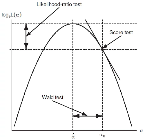
What’s the difference between likelihood ratio, Wald, and score tests?
The likelihood ratio test was developed by Jerzy Neyman and Egon Pearson (1928), the Wald test by Abraham Wald (1943), and the score test by C.R. Rao (1948) (Aitchison and Silvey (1958) developed the Lagrange Multiplier test which is equal to the score test).
The purpose of these tests is to compare two different (where one model is nested within the other) models to see which fits the data better. We assume the smaller model is true under the null hypothesis and that it is not the true model under the alternative. All three utilize the likelihood, though do so in different ways. The likelihood ratio test is the gold standard (most powerful), but the Wald and score tests may be computationally easier for certain model comparisons. The Wald and score tests generally perform poorly in small sample size scenarios. The Wald test is known to suffer from the Hauck-Donner effect.
- LRT: Fit both models and compare their likelihoods using \[\begin{align} LR &= -2log \left( \frac{L(model_1)}{L(model_2)}\right) \\ &= 2(logL(model_2) - logL(model_1)) \\ &\sim \chi^2_{df} \end{align}\] where \(model_1\) is the more restrictive model (fewer predictors; reduced), \(model_2\) the less restrictive model (more predictors; full), and the degrees of freedom for the test statistic is equal to the number of predictors included in \(model_2\) but not in \(model_1\). A small p-value indicates \(model_2\) is an improvement in fit.
- Wald: The Wald test only requires the larger model to be fit. It then tests how far the estimated coefficients are from zero (or whatever is used on the null hypothesis) in (asymptotic) standard errors and can allow multiple coefficients to be tested simultaneously. Thus we simply need to test that the parameters not included in the reduced model are simultaneously equal to zero. The resulting test statistic is also a \(\chi^2\) with degrees of freedom equal the number of predictors being tested. A small p-value indicates the larger model is an improvement in fit. Wald statistics are often the default values returned in statistical software because the standard error of the estimates (\(\sigma_{\hat{\beta}}\)) are available from the Hessian of the fitted model. The Z-test on \(\hat{\beta}/\sigma_{\hat{\beta}}\) provides p-values and normal confidence intervals.
- Score: The score test only requires the more restrictive model (reduced model). After fitting the model, the slope, or “score”, of the likelihood function (or log likelihood) can be evaluated at different values of coefficient values. If the score (slope) is very large, then we know that we are not close to the best value of the parameter, the MLE. The resulting test statistic is also a \(\chi^2\) with degrees of freedom equal the number of predictors being tested. A small p-value indicates the larger model is an improvement in fit.
References:
 Ref: John Fox, Applied Regression Analysis
What does it mean to fit a multivariable model? (Frisch-Waugh-Lovell theorem)
Assumptions
What are the assumptions of linear regression?
Validity
The data collected maps correctly to the questions of interest. The response variable reflects the phenomenon of interest and all relevant predictors are included.
Additivity
The effects of the covariates on the response are additive, along with the additive error term.
Linearity
The response variable is a deterministic component of a linear function of the predictors (linear in the parameters) plus an error term. The conditional means of the response are a linear function of the predictor variables.
No multicolinearity
The predictor variables are not a linear combination of each other. The design matrix \(\mathbf{X}\) is full rank.
Independence of errors
The errors from the regression line are independent (uncorrelated). In other words, the observations are independent from one another.
Equal variance of errors
The errors from the regression line have similar variability across the range of the response.
\(E[\epsilon \mid X] = 0\)
The errors have mean 0. This is also known as the strict exogeneity assumption. Exogeneity is violated when a confounding variable is not included.
Normality of errors
Normality of errors provides finite-sample guarantees for hypothesis testing and equivalence between the OLS estimate and the MLE.
How can you validate the validity assumption of linear regression?
- Use expert’s knowledge to determine the functional relationship with the response.
- If a relevant predictor variable is omitted:
- The OLS estimator of the coefficients will be biased (if correlated with each other).
- The variance of the error term will be biased.
- The covariance matrix of the coefficients will be biased.
- If an irrelevant predictor variable is included:
- The OLS estimator of the coefficients are unbiased (As the unneeded coefficient should be 0).
- The covariance matrix of the coefficients will be biased (increased).
- Before estimating coefficients, predict the sign of them. If they are different than expected, you may have omitted something correlated with that predictor variable.
References:
How can you validate the linearity assumption of linear regression?
- The residual vs. predicted plot should be symmetrically distributed around a horizontal line. If this relationship drifts away from zero, then the conditional expected response isn’t linear in the fitted values.
- Each individual predictor vs. observed plot should be symmetrically distributed around a linear line.
How can you validate the multicolinearity assumption of linear regression?
- Check pairwise correlations of predictor variables.
- Check for instability in coefficients and standard error of those estimates.
- Check the variance inflation factors (VIF)
- A VIF of 1.9 tells you that the variance of a particular coefficient is 90% bigger than what you would expect if there was no multicollinearity.
- VIFs are calculated by taking a predictor, and regressing it against every other predictor in the model. This gives you the \(R^2\) values for each predictor. \(VIF = \frac{1}{1-R^2_i}\)
How can you validate the independence assumption of linear regression?
The residual plots should look as if they were random noise.
- residuals vs. observation order
- residuals vs. time
- residuals vs. response
- residuals vs. each predictor
- ACF plot
Otherwise, verify that each observation in the data is independent of others.
How can you validate the equal variance assumption of linear regression?
The residual vs. fitted values plot should show constant variability.
How can you validate the normality of errors assumption of linear regression?
The QQplot should show a slope of one. QQplots can compare the distribution for any two vectors of data. For regression models, we usually look at a plot with the Normal distribution theoretical quantiles on the x-axis and the sample (residual) quantiles on the y-axis.
How can you fix the equal variance assumption of linear regression?
- Identify source of variation in residuals with residual vs. predictors plots.
- Use a variance stabilizing transformation. (Log or square root transform the response)
- Use a weighted least squares or robust regression.
- Use a generalized least squares (GLS) model.
References:
How can you fix the independence assumption of linear regression?
A linear mixed model (LMM) or generalized least squares (GLS) model may be a good choice as they provide methods to fit correlated errors.
How can you fix the linearity assumption of linear regression?
- You can try to identify source of nonlinearity with response vs. predictor plots.
- Log transformations on the response or predictors variables.
- Interaction effects between predictor variables.
- Polynomial terms for predictors.
- Spline terms for predictors.
How can you fix the normality of errors assumption of linear regression?
- Try transformations on response. (Log or square root)
- Try generalized least squares (GLS) model
- Try generalized linear model (GLM) model
What are the assumptions of logistic regression?
Validity
The data collected maps correctly to the questions of interest. The response variable reflects the phenomenon of interest (binary) and all relevant predictors are included.
Linearity
The log odds of the outcome (logit of outcome) are linearly related to each predictor variable.
Independence of observations.
Multicolinearity
The predictor variables are not a linear combination of each other.
What are the assumptions of Cox proportional hazards regression?
Validity
The data collected maps correctly to the questions of interest. The response variable reflects the phenomenon of interest (time to event or censoring) and all relevant predictors are included.
Linearity
The log hazard (or log cumulative hazard) of the outcome is linearly related to each predictor variable.
No Multicolinearity
The predictor variables are not a linear combination of each other.
Independence of observations
No event time bias
Each predictor variable is measured at or before baseline event time. When predictors, which are not a constant property of the observation, are measured after start of event time, then the observation had to remain event free until the time they were measured on that variable. This potential bias is known as event time bias (survival time bias or immortal time bias).
No informative censoring bias
This is generally defined by independence of censoring. subjects in subgroup \(g\) censored at time \(t\) should be representative of all subjects in subgroup \(g\) who remained at risk at time \(t\). i.e. random censoring conditional on each covariate.
Proportional hazards
There are no time by predictor interactions. The predictors have the same effect on the hazard function at all time points. The treatment effect should have the same relative difference in hazard compared to the control effect at all time points (their curves should not cross).
Specification
What conditions are required for causal interpretations in observational studies?
The conditions required for a causal analysis or conceptualization as a randomized experiment are:
- Consistency
- The values of treatment under comparison correspond to well-defined interventions that, in turn, correspond to the versions of treatment in the data.
- Exchangeability
- The conditional probability of receiving every value of treatment, though not decided by the investigators, depends only on measured covariates.
- Randomization produces exchangeability.
- Exogeneity is commonly used as a synonym for exchangeability.
- The treated, had they remained untreated, would have experienced the same average outcome as the untreated did, and vice versa.
- Positivity
- Each treatment value (treated vs. untreated) has a non-zero probability of being assigned, conditional on measured covariates, for each subject in a study. i.e. the probability is positive.
These conditions, and the specific functional form for identifiable effects, are usually untestable and can only be discussed with subject-matter knowledge and DAGs to justify the choices made.
Model specification can be performed under three general methods of inference:
- Description: How have things been?
- Prediction: What will happen next?
- Counterfactual/Causal: If we do X, what would happen to Y?
References:
- Consistency
What are DAGs?
DAGs (directed acyclic graphs) are useful tools to define the relationships between a set of covariates, exposure, and outcome variables. By making the structure and assumptions explicit, we can demonstrate whether the causal effect of the predictor of interest on the outcome is identifiable and, if so, which variables are required to ensure conditional exchangeability.
- Directed: points from cause to effect.
- Acyclic: no directed path can form a closed loop.
Common terminology used for DAG variables:
- X: Exposure, Treatment, Intervention, Primary Predictor, Counterfactual
- Y: Outcome, Response, Target
- Z: Confounder, Covariate, Secondary Exposure
- U: Unmeasured, Unobserved
References:
What is the backdoor criterion?
A set of covariates satisfy the backdoor criterion if all backdoor paths between the exposure and outcome are blocked by conditioning on the covariates and the covariates contain no variables that are descendants of the exposure. Conditional exchangeability is guaranteed if the backdoor criterion is satisfied.
The backdoor criterion is satisfied in two settings:
- No common causes of exposure and outcome.
- This means no backdoor paths need to be blocked. This is because the set of variables that satisfy the backdoor criterion is the empty set.
- This is representative of the marginally randomized experiment.
- There are no backdoor paths from the exposure to the outcome.
- Common causes of exposure and outcome but a subset of covariates that are non-descendants of the exposure suffice to block all backdoor paths.
- No unmeasured confounding.
- This is representative of the conditionally randomized experiment.
- Measured covariates are sufficient to block all backdoor paths from the exposure to the outcome
References:
- No common causes of exposure and outcome.
What is a backdoor path?
A backdoor path is a non-causal path from an exposure variable to an outcome variable. In other words, if we removed the direct paths that flowed from the exposure to the outcome, are there any other lines left that connects these two variables? Or, the path from the exposure to the outcome that links the exposure and outcome through their common cause Z.
Backdoor paths bias the effect estimates that we want (total or direct effect), thus we wish to create a model that blocks backdoor paths. Backdoor paths are blocked when we adjust for confounders or we do not adjust for colliders.
References:
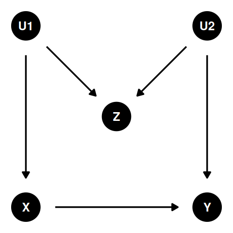
What is a confounding variable?
Confounding is systematic error introduced into a statistical model when a third variable interferes with the exposure (predictor variable of interest) and outcome variables.
Covariates included in the model should be
- Associated with the predictor of interest.
- Cause the outcome (the covariate influences the outcome and not the other way around).
- Not located between the exposure and outcome on the causal pathway.
For example:
- Bad: exposure -> covariate -> outcome
- Good: covariate -> exposure -> outcome
- Consider a study about grades and alertness in class. Amount of sleep is associated with alertness and also could be regarded as a causal influence on grades. Thus amount of sleep is a good (confounding) covariate to adjust for.
- Amount of sleep (confounder) -> alertness (predictor) -> grades (outcome)
So the steps to follow are:
- Identify variables which may cause the outcome.
- Identify the variables in step 1 that are associated with the exposure.
- Make sure the variables in step 2 are not on the causal pathway (the exposure is not causing the covariate)
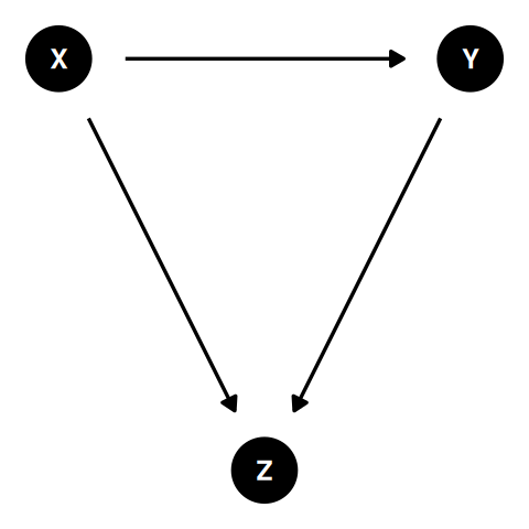
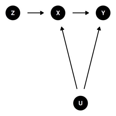
What is a collider variable?
Collider bias occurs when two variables (the outcome and exposure) independently cause a third variable (a covariate) and this third variable is included in the model. Controlling for a collider will open the backdoor path, thereby introducing bias.
Collider’s are path specific. The path from the exposure to the outcome must have a third variable in the middle with arrows (one from the exposure side and one from the outcome side) pointing to it.
References:
What is M-bias?
M-bias (named after the shape of the DAG) is caused by adjusting for a third covariate which is directly caused by two (potentially unobserved) ancestors of the exposure and outcome, thereby turning it into a collider [1]. Selection bias is a common example leading to M-bias.
What is an instrumental variable?
Let \(y = bx + u\) where X and Y are observed variables and U is an error term. If X and U are correlated, then \(b\) cannot be estimated without bias. However, if there was a third observed variable, Z, that was correlated with X and uncorrelated with U, then \(b = \frac{r_{yz}}{r_{xz}}\).
For example, in a clinical trial, Z might be the treatment assigned to a subject, X is the treatment actually received, and Y is the outcome.
References:
What is mediation?
A variable (Z) is a mediator if it lies between an exposure (X) and the outcome (Y) on the causal path: X -> Z -> Y.
- The indirect effect of X on Y is the product of the coefficients from X to Z and from Z to Y. In other words, the change in Y when Z increases by one unit and X remains constant.
- The direct effect of X on Y is the coefficient of the path from X to Y only. In other words, the change in Y when X increases by one unit and Z remains constant.
- The total effect of X on Y is the sum of the indirect and direct effects.
Mediation analysis traditionally follows from the paper by Baron and Kenny (1986) [1]:
- Verify that X is a significant predictor of Y:
lm(Y ~ X). If it is not, no ground for mediation. - Verify that X is a significant predictor of Z:
lm(Z ~ X). If it is not, no ground for mediation. - Verify that Z is a significant predictor of Y and the coefficient estimate for X is smaller in absolute value.
lm(Y ~ X + Z) - If the effect of X on Y completely disappears, Z fully mediates between X and Y (full mediation). If the effect of X on Y still exists, but in a smaller magnitude, Z partially mediates between X and Y (partial mediation). If the effect of X on Y is just as larger or larger, Z does not mediate between X and Y.
- Use Preacher and Hayes (2004) [2] bootstrapping method to generate confidence intervals on the mediation effect. ACME is the indirect effect of Z (total effect - direct effect) and tells us if our mediation effect is significant.
library(mediation); mediate()
(Review modern thoughts on this method)
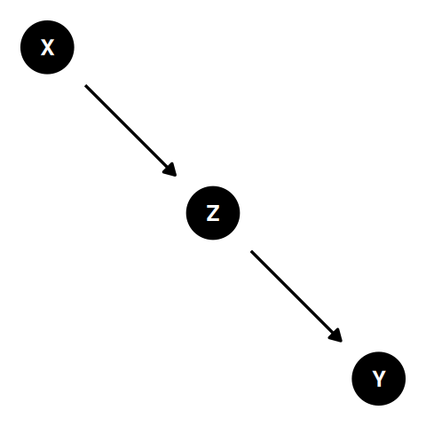
What is moderation?
A variable (Z) is a moderator if it is an effect modifier of X in the relationship between the exposure (X) and the outcome (Y). Moderation and mediation are easy to confuse. Moderation tests for when the relationship is modified versus mediation which tests for how/why the relationship is modified. Use a LRT or Wald test on the interaction relationship.
What is interaction/effect modification?
Statisticians often use the word interaction to refer to a product term in a linear model without reference to causality. It is little more than observing the effect of one predictor variable (X) on the response variable (Y) changing at different levels of another predictor variable (Z). However, both interaction and effect modification also have distinct causal specific definitions.
Effect modification is defined in terms of the effect of one intervention (X) on an outcome (Y) that varies across strata of a second variable (Z). Interaction is defined in terms of the effects of 2 interventions (X1 and X2) on an outcome (Y).
Below is an example of effect modification in the absence of interaction. The absence of interaction is a direct result of the structure of the DAG.
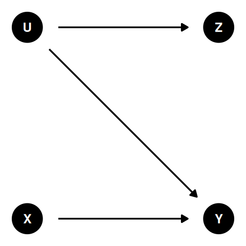
Below is an example of interaction in the absence of effect modification. The absence of effect modification only applies if we assume/show that the indirect effect of Z cancels out the direct effect of Z.
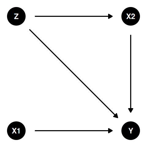
References:
How would you perform exploratory model selection?
The best model selection is through pre-specification using existing expert knowledge. However, this is not always feasible. Thus, we are left with data-dependent model building, which is subject to its own set of issues, including:
- replication stability
- selection bias
- omitted variable bias
- underestimation of variance
- overestimation of the predictive ability
Below, I outline the steps to determine if the data, and any given model selection technique, is capable of selecting a seemingly robust model. However, it may result in selecting a bad model if the inclusion of two (or more) variables depends on each other. It may be that one of two (or more) variables is included in each of the replications, but the individual inclusion frequency is not much higher than 50%. Thus, based on their inclusion frequencies, neither variable maybe judged important.
- Statistical methods cannot distinguish between spurious and real associations between variables. So we first need to pre-specify a set of candidate covariates for which domain expertise would assume association with the response variable.
- Since this usually hard to do, consider the results from unsupervised learning methods such as hierarchical clustering or PCA.
- Choose an appropriate model selection method.
- Traditional
- Univariate screening
- Backward selection
- Change in coefficient
- If elimination of standardized coefficient results in more than X% change in other predictor of interest, then it will not be removed.
- Penalized likelihood
- Lasso
- Elastic net
- Adaptive Lasso
- Boosting
- Gradient boosting
- Likelihood boosting
- Model free
- Feature ordering by conditional independence (FOCI).
- Traditional
- Use the nonparametric bootstrap to generate repeated runs of the selection algorithm.
- Assess the stability of model selection through
- Variable inclusion frequency
- Model selection frequency
- If you do not see stable results, then it is unlikely that a data based model selection method will return interpretable results.
The traditional K-fold cross-validation approach to model selection and evaluation of performance looks like:
- Divide data into \(K\) folds at random.
- For each fold \(k = 1, 2, \dots, K\)
- Find a subset of “good” predictors (univariable, stepwise, FOCI, etc.) that show association with the outcome using only the remaining \(k-1\) folds of data.
- Fit the models using the selected predictors on only the remaining \(k-1\) folds of data.
- Evaluate the model performance on the test set \(k\).
- Calculate the average performance across all \(K\) folds.
The important step here is that the test set is left out before the outcome variable variable is used for predictor variable selection.
References:
- https://doi.org/10.1186/s41512-020-00074-3
- https://doi.org/10.1002/bimj.201700067
- Chapter 7, the elements of statistical learning
How would you perform Bayesian model selection?
Obviously, do what Aki Vehtari recommends.
Performance
What is cross validation?
Cross validation is a method to evaluate the performance of a statistical model on unseen data. Common methods include K-fold cross validation and bootstrap resampling.
Cross validation can be used for both model selection and assessment of model performance. However, care is needed when you wish to estimate both. Nested cross validation or the double bootstrap should be used for this situation as it provides an estimate of the unbiased model error (i.e. “cross-validatory assessment of the cross-validatory choice”).
Cross validation is used to evaluate the procedure for model building. Once the characteristics of the procedure is known, then the final prediction model is built using the full dataset.
References:
What is K-fold cross validation?
- Randomly divide (or stratify) the dataset into \(K\) folds.
- For each fold \(k = 1, \dots, K\)
- Let fold \(k\) be the test set and the remaining \(K-1\) folds used for training.
- Fit the model on the training set.
- Note: ‘model’ is referring the learning method, variable selection method, and tuning parameter/hyperparameter choice.
- Calculate the performance estimate \(S_{k}\) by evaluating the model on test set \(k\).
- Calculate the mean prediction performance estimate \(\bar{S}\). \[\bar{S} = \frac{1}{K} \sum_1^{K} S_{k}\]
- Report the cross-validated prediction performance \(\bar{S}\).
- Fit the model on the original dataset.
k=n results in LOO-CV (leave one out cross validation).
Page 184, An Introduction to Statistical Learning:
Typically, given these considerations, one performs k-fold cross-validation using k=5 or k=10, as these values have been shown empirically to yield test error rate estimates that suffer neither from excessively high bias nor from very high variance.
What is bootstrap cross validation?
- Fit the model to the original data and calculate the apparent performance estimate \(S_{app}\).
- For \(n = 1, ..., N\)
- Generate a bootstrapped dataset (with replacement) from the original data.
- Fit the model to resample \(n\).
- Calculate the apparent bootstrapped performance estimate \(S_{n_{boot}}\).
- Calculate an additional performance estimate \(S_{n_{boot:orig}}\) by evaluating the bootstrapped model on the original data.
- Calculate the optimism of the apparent performance estimate. \[O = \frac{1}{N} \sum_{1}^{N} (S_{n_{boot}} - S_{n_{boot:orig}})\]
- Calculate the optimism adjusted performance estimate. \[S_{adj} = S_{app} - O\]
- Report the model’s validated performance estimate using \(S_{adj}\).
The bootstrap CV method can be biased, especially for cases when N<P or when using discontinuous performance measures. This is because the original dataset shares observations between the ‘test’ set and ‘training’ sets. Overfit predictions will be unrealistically good. The leave-one out bootstrap, .632 bootstrap, and .632+ bootstrap were developed to alleviate these issues. However, the naive version is relatively common in use due to 1) it’s simplicity and 2) when used for model selection (performance estimates are not the primary outcome) consistent bias will still lead to a consistent choice for optimal model?
References:
- https://doi.org/10.1080/01621459.1997.10474007
- Chapter 7, the elements of statistical learning
What cross validation method applies to time series data?
Since time series data has inherent serial correlation and potential non-stationarity, internal cross validation is not as straight forward as with traditional data modeling. The naive approach is to simply hold out a section from the end of the series to use for evaluation.
Standard K-fold CV is ok to use for strictly autoregressive (predictors are lagged values of the response) time series [1].
Time series CV (AKA forward chaining, rolling origin CV) can be used for the general case. For this procedure, the sample is split in to N sets chronologically, then models are fit and tested rolling forward into time and performance summaries are averaged like usual [2]. For example:
- training (1), test (2)
- training (1, 2), test (3)
- training (1, 2, 3), test (4)
- training (1, 2, 3, 4), test (5)
This is known as one-step time series CV. Multi-step time series CV could look like:
- training (1), test (3)
- training (1, 2), test (4)
- training (1, 2, 3), test (5)
What are the differences between training, validation, and test sets?
- Training set
- Used to fit competing models.
- Validation set
- Used to assess performance of competing models and then select the top performer.
- Test set
- Used to assess the performance of the selected model.
The algorithm for repeated K-fold cross validation uses only training and test sets and is implemented as:
- For each repeat \(n = 1, \dots, N\)
- Randomly divide (or stratify) the dataset into \(K\) folds.
- For each fold \(k = 1, \dots, K\)
- Let fold \(k\) be the test set and the remaining \(K-1\) folds used for training.
- Fit the model on the training set.
- Note: ‘model’ is referring the learning method, variable selection method, and tuning parameter/hyperparameter choice.
- Calculate the performance estimate \(S_{kn}\) by evaluating the model on test set \(k\).
- Calculate the mean prediction performance estimate \(\bar{S}\). \[\bar{S} = \frac{1}{KN} \sum_1^{N} \sum_1^{K} S_{kn}\]
- Report the cross-validated prediction performance \(\bar{S}\).
- Fit the model on the original dataset.
The algorithm for repeated nested K-fold cross validation uses training, validation, and test sets, and is implemented as:
- For each repeat \(n = 1, \dots, N\)
- Randomly divide (or stratify) the dataset into \(K\) folds.
- For each fold \(k = 1, \dots, K\)
- Let fold \(k\) be the test set and the remaining \(K-1\) folds used for cross-validation.
- Recombine the remaining \(K-1\) folds and randomly divide (or stratify) them into \(J\) folds.
- For each fold \(j = 1, \dots, J\)
- Let fold \(j\) be the validation set and the remaining \(J-1\) folds used for training.
- For each model \(i_{inner} = 1, \dots, I\)
- Fit model \(i_{inner}\) on the training set.
- Note: ‘model’ is referring the unique combination of learning method, variable selection method, and tuning parameter/hyperparameter choice.
- Calculate the performance estimate \(S_{i_{inner}jkn}\) by evaluating model \(i_{inner}\) on the validation set \(j\).
- Fit model \(i_{inner}\) on the training set.
- For each model \(i_{outer} = 1, \dots, I\)
- Fit model \(i_{outer}\) on the cross-validation set.
- You can construct a more efficient algorithm which does not require fitting the unselected models.
- You may carry over the hyperparameters estimated in the inner loop.
- Calculate the performance estimate \(S_{i_{outer}kn}\) by evaluating model \(i_{outer}\) on the test set \(k\).
- Fit model \(i_{outer}\) on the cross-validation set.
- Calculate the mean prediction performance \(\bar{S}\) from inner loop \((j)\). For each model \(i_{inner}\), \[\bar{S}_{i_{inner}} = \frac{1}{JKN} \sum_1^{N} \sum_1^{K} \sum_1^{J}(S_{i_{inner}jkn})\]
- Determine which model has best prediction performance and proceed using selected model method \(i\).
- Calculate the mean prediction performance from outer loop \((k)\). For selected model \(i_{outer}^{top}\), \[\bar{S}_{i_{outer}^{top}} = \frac{1}{KN} \sum_1^{N} \sum_1^{K}(S_{i_{outer}^{top}kn})\]
- Report the cross-validated prediction performance \(\bar{S}_{i_{outer}^{top}}\).
- Use the selected method to fit the final model on the original dataset.
References:
- Training set
What is internal model validation?
Internal validation means reusing parts or all of the data on which a model was developed to assess the amount of (likely) overfitting and correct for the amount of ‘optimism’ in the performance of the model.
This is generally done through cross validation and model performance summaries such as \(R^2\), calibration, and discrimination are assessed.
See notes on bootstrap cross validation for implementation.
What is external model validation?
External model validation means assessing the performance of a model already developed when applied to an independent dataset.
Generally, independent datasets have one or more of the following properties:
- Temporal differences
- Data may be collected from the same locations, but over different periods of time.
- Geographic differences
- Data was collected from different locations.
- Institutional differences
- Data was collected from an organization not connected with the original source.
If the external sample is very similar to the original sample, the assessment is for reproducibility rather than for transportability.
Steps:
- Compare variable characteristics of original sample and new sample.
- Compare results of model selection algorithm from original model and the model based on the external data.
- Use the original model and apply it to the new sample, then calculate apparent prediction performance.
- Compare prediction performance for
- original model, original data, apparent
- original model, original data, optimism adjusted (old model internal validation)
- original model, new data, apparent (old model external validation)
- Determine if differences are from overfitting, missing predictors, differences in data capture, extrapolation, etc..
- Compare prediction performance for
- If warranted, combine original and new data, then re-fit a new model.
- Compare prediction performance for
- combined model, combined data, apparent
- combined model, combined data, optimism adjusted (new model internal validation)
- Compare prediction performance for
Royston and Altman suggest:
- Regression on linear predictors of external data
- Measure of calibration.
- Compute the linear predictors from original model fit on external data, then regress X = linear predictors on Y = outcome from external data.
- If the slope in the validation dataset is < 1, discrimination is poorer. If it is > 1, discrimination is better
- Likelihood ratio test for slope=1 is recommended, but may be anti-conservative since it does not allow for uncertainty in the estimated regression coefficients that constitute the linear predictor.
- Risk groups for survival
- Calculate linear predictor for each patient and split into quantile based risk groups.
- Create Kaplan-Meier plot stratified by risk group.
- Are groups well separated? Implies good discrimination.
- Do not use logrank test for differences…
- Are groups well separated? Implies good discrimination.
- Use Cox model to derive predicted survival for each group.
- Create survival plot with Cox-based predicted survival curve and observed Kaplan-Meier curves.
- Are curves overlapping? Implies good calibration.
See the TRIPOD statement
- Temporal differences
How would you assess performance of Bayesian models?
In summary, use LOO CV.
- WAIC is computationally more complex and harder to detect failure compared to LOO.
- WBIC is computationally more complex than WAIC.
- DIC is for posterior mean point estimation, not full Bayesian inference.
- AIC is for maximum likelihood, not full Bayesian inference.
References:
What are some model fit summaries for linear regression?
- \(R^2 = 1-\frac{SSE}{SST}\)
- The proportion of variability in the response explained by the model.
- Adjusted \(R^2 = 1 - \frac{SSE / (n-d-1)}{SST / (n-1)}\)
- where \(d\) is the number of parameters in the model.
- \(\text{RMSE} = \sqrt{\frac{1}{n} \sum_{i=1}^{n} (y_i - \hat{f}(x_i))^2} = \sqrt{\frac{SSE}{d.f.}}\)
- The standard deviation of the unexplained variance (same units as response). The typical difference between the observed and fitted values.
- Mallow’s \(C_p = \frac{1}{n} (SSE + 2d\hat{\sigma}^2)\)
- \(\text{AIC} = -2logL+2d\)
- If OLS conditions are satisfied, then \(C_p = \text{AIC}\).
- Optimism adjusted calibration curve
- \(R^2 = 1-\frac{SSE}{SST}\)
What are some model fit summaries for logistic regression?
- ROC-AUC
- The ROC-AUC is the probability that the model ranks a random positive observation more highly than a random negative observation.
- Concordant pairs
- The percent of concordant, discordant, and tied pairwise comparisons. The concordant percent is proportional to the AUC. AUC = percent concordant + 0.5*percent tied.
- Brier score
- Quadratic scoring rule
- The squared differences between actual binary outcomes Y and predictions p. \((y-p)^2\)
- Analogous to mean squared error
- The Brier score for a model can range from 0 for a perfect model to 1 if predicting exactly wrong all the time. For an outcome that has 50% prevalence, a non-informative model (‘coin flip’ correct) would result in a brier score of 0.25. The expected Brier score for non-informative models is \(max(brier)=x(1-x)^2+(1-x)x^2\), for population prevalence \(x\).
- Similar to Nagelkerke’s \(R^2\), the scaled version of Brier’s score can be similar to Pearson’s \(R^2\). \(R^2_{\text{Brier}} = 1 - \frac{Brier}{max(Brier)}\) will range between 0-1.
- Calibration
- Mean calibration == calibration-in-the-large
- Calibration intercept
- Weak calibration
- Combination of calibration intercept and calibration slope
- Proper loss functions lead to apparent intercept = 0 and slope = 1. CV’d values have different intercept and commonly slope < 1.
- Calibration slope == linear shrinkage factor
- Need to report calibration intercept together with calibration slope.
- Moderate calibration
- Smoothed calibration plot of observed vs. predicted outcomes.
- Pointwise calibration suffers from same issues as dichotomization.
- Strong calibration
- Assessment of observed vs. predicted outcomes over multidimensional covariate space.
- Not possible for any real situation
- Mean calibration == calibration-in-the-large
- Classification table
- Goodness of fit test (GOF)
- le Cessie-van Houwelingen-Copas-Hosmer unweighted sum of squares test for global goodness of fit. [1]
- ROC-AUC
When is a model underfit?
A model is underfit when it assumes the relationship between the explanatory variables and the response variable is more simple than it actually is.
When is a model overfit?
A model is overfit when the model predictions match very closely with the observed data, but perform poorly on new data.
Other
What is logistic regression?
Logistic regression is a logit-link generalized linear model that will generate predicted probabilities for the binary response variable using a linear combination of predictor variables.
How would you interpret the coefficient for a continuous predictor in linear regression?
The coefficient of a continuous predictor represents the additive change in the response variable for each 1 unit change in the predictor.
How would you interpret the coefficient for a categorical predictor in linear regression?
For treatment/dummy encoded categorical variables, each coefficient represents the additive unit change in the response variable relative to the reference level of the categorical variable.
How would you interpret the coefficient for a continuous predictor in logistic regression?
- The raw coefficient of a continuous predictor represents the additive change in log odds of the response for a 1 unit change in the predictor.
- For example: A 1 unit increase in the predictor is associated with the log odds increasing by 0.25.
- The exponentiated coefficient of a continuous predictor represents the multiplicative change in odds of the response for a 1 unit change in the predictor (odds ratio).
- For example: A 1 unit increase in the predictor is associated with the odds increasing by 50% (or odds increasing 1.5 times).
- The raw coefficient of a continuous predictor represents the additive change in log odds of the response for a 1 unit change in the predictor.
How would you interpret the coefficient for a categorical predictor in logistic regression?
For treatment/dummy encoded variables:
- The raw coefficient represents the additive change in log odds of the response relative to the reference level of the categorical variable.
- For example: compared to level A, level B is associated with the log odds increasing by 0.25.
- The exponentiated coefficient represents the multiplicative change in odds of the response relative to the reference level of the categorical variable (odds ratio).
- For example: Compared to level A, level B is associated with the odds increasing by 50% (or odds increasing 1.5 times).
- The raw coefficient represents the additive change in log odds of the response relative to the reference level of the categorical variable.
What is the risk ratio?
- Relative risk = risk ratio.
- The ratio of the probability of an outcome in an exposed group to the probability of an outcome in an unexposed group.
- We generally prefer Odds Ratios as the RR does a poor job when baseline risk varies, and baseline risk tends to vary a lot.
- Risk ratios should not be used in case-control studies.
If we found that 17% of smokers develop lung cancer and 1% of non-smokers develop lung cancer, then we can calculate the relative risk of lung cancer in smokers versus non-smokers as: Relative Risk = 17% / 1% = 17
Thus, smokers are 17 times more likely to develop lung cancer than non-smokers.
What is the odds ratio?
- The ratio of the odds of an outcome in an exposed group to the odds of an outcome in an unexposed group.
- We generally prefer Odds Ratios as the RR does a poor job when baseline risk varies, and baseline risk tends to vary a lot.
- When an event is rare, then odds ratios approximate ratios of probabilities (the risk ratio).
- When an event is not rare, the odds ratio is larger compared to the risk ratio.
- Can be used in case-control studies.
- In contrast to identity and log-link (risk ratio) GLM models, the logit-link model results in non-collapsible odds ratios.
If 17 smokers have lung cancer, 83 smokers do not have lung cancer, one non-smoker has lung cancer, and 99 non-smokers do not have lung cancer, the odds ratio is calculated as follows:
- Odds in exposed group = (smokers with lung cancer) / (smokers without lung cancer) = 17/83 = 0.205
- Odds in not exposed group = (non-smokers with lung cancer) / (non-smokers without lung cancer) = 1/99 = 0.01
- Odds ratio = (odds in exposed group) / (odds in not exposed group) = 0.205 / 0.01 = 20.5
- This group of smokers has 20 times the odds of having lung cancer than non-smokers.
What are collapsible vs non-collapsible estimates?
- Collapsible means that adjusting for other covariates which are uncorrelated with the covariate of interest will not change its estimated value (although it may change the SE).
- Non-collapsible means that adjusting for other covariates which are uncorrelated with the covariate of interest will change its estimated value.
- Odds ratios [1] and hazard ratios [2] are two common non-collapsible estimates.
What is supervised learning?
Supervised learning is when you have measurements on a set of predictor variables and response variable so that you can create a function, Y = f(X), that best explains the relationship between them. Regression model = supervised learning.
What is unsupervised learning?
Unsupervised learning is when you have data on a set of variables and would simply like to find underlying structure or patterns within this set of data. Clustering/Association = unsupervised learning.
What model would you use for an ordered response variable?
- Proportional odds model.
- AKA cumulative logit model with proportional odds assumption.
- \(log\left( \frac{P(Y \leq j)}{P(Y > j)} \right) = log\left( \frac{P(Y \leq j)}{1-P(Y \leq j)} \right)\), for ordered response Y with levels \(j = 1, \dots, J\).
- \(logit(P(Y \leq j)) = log\left( \frac{P(Y \leq j)}{P(Y > j)} \right)\).
- \(P(Y=j) = P(Y \leq j) - P(Y \leq j-1)\)
- Continuation ratio model.
- Observations assumed to pass through lower levels to reach higher levels.
- The probability of being in category j conditional on being in categories greater than j.
- \(log \left( \frac{P(Y = j)}{P(Y > j)} \right)\)
- Adjacent categories model.
- \(log \left( \frac{P(Y = j)}{P(Y = j+1)} \right)\)
References:
- Proportional odds model.
What is best subset regression?
Best subset selection is L0 penalization. It requires fitting separate models for each possible combination of the predictors. Unfortunately this requires \(2^p\) models, thus is computationally unfeasible once \(p>40\) (\(2^{20}\) ~ million, \(2^{30}\) ~ billion, \(2^{40}\) ~ trillion). In practice, algorithms which search a smaller set of models are used instead.
- Forward stepwise selection
- Starts with a zero predictor model and adds each predictor one at a time.
- Requires \(1+p(p+1)/2\) models.
- Can still be used if \(n<p\).
- Backward stepwise selection
- Starts with the full model and removes the least informative predictor one at a time.
- Requires \(1+p(p+1)/2\) models.
- Cannot be used if \(n<p\)
- Hybrid stepwise selection
- Forward stepwise selection
What is Lasso regression?
Lasso regression uses L1 penalization. The penalization is proportional to the sum of the absolute value of the regression coefficients. The shrinkage is by a fixed amount and may shrink some regression coefficients to ~0. LARS (Least angle regression) is the simplest implementation of Lasso.
- Cost = loss function + penalty term
- Cost = \(\sum_{i=1}^n \left( y_i - \beta_0 - \sum_{j=1}^p \beta_jx_{ij} \right)^2 + \lambda \sum_{j=1}^p |\beta_j|\)
Generally, we select the tuning parameter value \(\lambda\) for which the cross-validation error is smallest. larger values of \(\lambda\) will be more likely to force coefficients to zero.
What is Ridge regression?
Ridge regression uses L2 penalization. The penalization is proportional to the sum of the squared regression coefficients. The shrinkage is by a proportional amount, so does not shrink some coefficients to zero as in Lasso.
- Cost = loss function + penalty term
- Cost = \(\sum_{i=1}^n \left( y_i - \beta_0 - \sum_{j=1}^p \beta_jx_{ij} \right)^2 + \lambda \sum_{j=1}^p \beta_j^2\)
Generally, we select the tuning parameter value \(\lambda\) for which the cross-validation error is smallest. larger values of \(\lambda\) will be more likely to push coefficients towards zero.
What is ensemble learning?
Ensemble methods combine several models into one model. Predictive performance from an aggregated set of diverse models is often better than what is possible from trying to choose a single model.
Ensemble methods include:
- Bagging
- Boosting
- Model averaging
- Stacking
What is bagging?
Bagging was introduced by Leo Breiman in 1996. It’s essentially bootstrap averaging (Bootstrap Aggregating) of model predictions. Bagging is useful for lowering the variance of high-variance models (i.e. smoothing out their predictions).
- Sample k data sets \(D_1, ..., D_k\) from D with replacement (Bootstrap)
- Increasing k eventually leads to diminishing returns.
- For each sample, fit the model.
- Average the model estimates.
Random forests are a popular model implementation of the bagging algorithm.
References:
- Sample k data sets \(D_1, ..., D_k\) from D with replacement (Bootstrap)
What is boosting?
Boosting refers to the family of algorithms which sequentially train a set of models using the data that was misclassified by the previous model. Each individual model in the sequential process is said to be a weak learner, and the combination of these weak learners boosts the combined complexity of predictions.
Gradient boosting is a common boosting method and XGBoost is a popular implementation.
References:
What is random forests?
Random forests is a classification method based on decision trees. The data is resampled using independent bootraps, a random set of variables is selected, and a new classifier is fit on each. Since any individual decision tree is prone to overfitting, bagging is used to average predictions for smoothed model estimates. Each individual tree is uncorrelated. Unlike boosting (which is sequential), random forests grows trees in parallel. Since trees can be fit in parallel, it’s usually faster than boosting methods.
Tuning parameters:
- Number of trees (The more the better)
- How big a tree can grow (bagging counteracts overfitting, so bigger is usually better)
- Minimum number of samples per leaf (Usually start with 1, can try increasing to 2, 3, …)
- Maximum number of variables to consider
References:
What is gradient boosting?
Gradient boosting adds new models to the ensemble through a sequential process. At each iteration, a “weak” model contributes an updated parameter estimate to the ensemble and the gradient of the loss function is updated. More weight is added to poorly fit observations so that future model iterations may minimize these errors.
Decision trees are often used as the backend modeling solution since the functional form of the regressor/classifier can evolve over sequential fits. OLS isn’t a valid ‘classifier’ since the sum of sequential linear models can be represented as a single, larger model more efficiently (automatically provides the best estimate for \(\beta\)). Thus, if we already know what the (simple) functional form should be, there is little reason to use gradient boosting.
Tuning parameters:
- Number of trees
- Learning rate
- Tree complexity
References:
What is pruning a decision tree?
When you remove a sub-node of a decision node for the purposes of simplifying the complexity of the classifier.
What is the class imbalance problem?
The class imbalance problem is the observation that some ‘classification’ algorithms do not perform well when the proportion of one class is much smaller than the other class.
This problem is really a result of three separate issues:
- Assuming that accuracy is an appropriate metric of model fit. i.e. you assign an equal cost to false positive and false negatives.
- Assuming that the test distribution matches the training distribution when it actually does not.
- The frequency of the minority class is too small to make reliable inference on.
Using the wrong model fit measure (accuracy) or algorithms that do not model probabilities (SVM, tree methods) are the main problem in this scenario.
This scenario is not a problem if you use a model that generates predicted probabilities based on a proper loss function and have enough observations in the smaller class.
References:
What are precision, recall, sensitivity, and specificity?
- Precision = Positive predictive value
- Recall = Sensitivity
- Precision = P(truth is positive | estimate is positive) = What is the probability that this is a real hit given my classifier says it is?
- Recall = P(estimate is positive | truth is positive)
- Specificity = P(estimate is negative | truth is negative)
- ROC uses sensitivity and specificity, and they condition on the true class label.
What is an ROC curve?
The receiver operating characteristic (ROC) curve is a graphical representation of the contrast between true positive rates and false positive rates at various thresholds.
When should you use a ROC or PR curve?
- Receiver operator characteristic (ROC)
- Precision Recall (PR) curve
- PR curve: How meaningful is a positive result from my classifier given the baseline probabilities of my problem?
- ROC: How well can this classifier be expected to perform in general, at a variety of different baseline probabilities?
References:
What is the ROC-AUC or c-index?
The AUC (or concordance index) is the probability that the model ranks a random positive observation more highly than a random negative observation. It is a measure of discrimination, but doesn’t contain information about calibration.
AUC = percent concordant + 0.5*percent tied
When predicting {1} for event outcomes {0, 1}:
- Concordant pairs
- An outcome of 1 has a higher predicted probability than an outcome of 0.
- Discordant pairs
- An outcome of 1 has a lower predicted probability than an outcome of 0.
- Tied pairs
- An outcome of 1 has the same predicted probability as an outcome of 0.
- Concordant pairs
What is the confusion matrix?
A matrix with actual classification as columns and predicted classification as rows.
actual + actual - predicted + a (TP) b (FP) predicted - c (FN) d (TN) - True positive(TP) — Correct positive prediction
- False positive(FP) — Incorrect positive prediction
- True negative(TN) — Correct negative prediction
- False negative(FN) — Incorrect negative prediction
What are the common binary diagnostic summaries?
actual + actual - predicted + a (TP) b (FP) predicted - c (FN) d (TN) - Apparent prevalence \(= P(\text{predicted} +) = \frac{a+b}{N}\)
- True prevalence \(= P(\text{actual} +) = \frac{a+c}{N}\)
- Sensitivity \(= P(\text{predicted} + \mid \text{actual} +) = \frac{a}{a+c}\)
- Specificity \(= P(\text{predicted} - \mid \text{actual} -) = \frac{d}{b+d}\)
- Overall accuracy \(= P(\text{predicted was correct}) = \frac{a+d}{N}\)
- Positive Predictive Value \(= P(\text{actual} + \mid \text{predicted} +) = \frac{a}{a+b}\)
- Negative Predictive Value \(= P(\text{actual} - \mid \text{predicted} -) = \frac{d}{c+d}\)
- Proportion of false positives \(= P(\text{predicted} + \mid \text{actual} -) = \frac{b}{b+d}\)
- Proportion of false negatives \(= P(\text{predicted} - \mid \text{actual} +) = \frac{c}{a+c}\)
What is deep learning?
Deep learning refers to a neural network model that can be used to make flexible nonlinear predictions using a large number of features.
Why should a linear model include an intercept term?
A linear model should include an intercept term so that slope estimates are not unintentionally biased.
Even if we believe the intercept to be zero, there may be threshold input levels that are best estimated including the intercept.
If two predictor variables have zero correlation, can we consider them statistically independent?
Not necessarily. Lack of linear correlation doesn’t mean they are independent. They might be nonlinearly dependent, such as x and x^2. (Hint: verify assumptions before answering.)
What is the difference between a zero-inflated model vs. hurdle model?
Sometimes outcomes contain more zeros than what would be expected under traditional distributional assumptions. If a model’s lack of fit is from too many zeros, we might refer to the data being ‘zero-inflated’.
This type of data arises from three common data generating mechanisms:
- Hurdle data
- Data generating process 1: Observations which will always be zero.
- Data generating process 2: Observations which will always be non-zero (>0)
- Zero-inflated data
- Data generating process 1: Observations which will always be zero.
- Data generating process 2: Observations may be 0 or non-zero.
- Single process data
- Data generating process: Observations may be 0 or non-zero.
Zeros can be ‘structural’, meaning there is some process which prevents a non-zero value being realized, or they can be ‘sampling’, meaning that a zero is realized by chance of the underlying distribution.
An example of zero-inflated data would be the number of visits to a dentist in a year. The first data generating process would be people who actively avoid going to the dentist vs. those who generally go. The second data generating process would be those who generally go, but could possibly not see the dentist because of schedule conflicts or other reasons of causing a zero.
An example of hurdle data would be the number of drinks on a typical drinking day. Some people abstain from drinking thus by definition would be zero. People who do not abstain by definition would have 1+ drinks.
We call hurdle and zero-inflated models ‘mixture models’ since we need to model the data as a mixture of two separate distributions. Typically a binomial distribution is used for the zero/non-zero process and a Poisson or negative binomial is used for the 0+ process. The hurdle model uses whats called a ‘truncated’ Poisson or negative binomial model which modifies the model to condition on only positive outcomes.
If there is only a single process generating the data, then using an alternative model such as an negative binomial, ordinal, or Tweedie GLM may provide good fit.
References:
- Hurdle data
What is a principled way to handle missing data?
- Double check and verify missingness.
- Look for patterns in the missingness, such as between the missing cases and other observed data.
- If you believe the data are MCAR and the sample size of the final model is sufficient, use complete case analysis. You can argue the validity of the MCAR assumption by creating a ‘table one’ grouped by missingness and compare the distribution of other Ys and Xs. If there are differences in distribution, we cannot say if the missingness is due to MAR or MCAR. Keep in mind that lack of any differences does not guarantee MCAR, so do not place too much importance on it compared to subject matter expertise.
- If missing in X, and you have data that may explain why those values are missing (MAR), use multiple imputation (or a ‘nice’ single imputation method if simplicity is more important) where the imputation model includes both Y and the variables related to missingness.
- If missing in Y, or X and Y, and you have data that may explain why those values are missing, use multiple imputation. It is important to use subject matter expertise to define the structure of the imputation mode (make sure to capture nonlinearities and interactions.). If only Y is MAR or MCAR, [1] indicates that MI has little benefit compared to CCA, unless an auxiliary variable is available for filling in Y. If missing in X and Y, then follow the approach of [2].
- For all other cases, your choices are
- Use multiple imputation and pray your results are not significantly biased
- Collect a new sample that will not be biased from missing values
- Do not conduct the analysis.
- MCAR (NDD)
- If the probability of being missing is the same for all cases and is unrelated to the data, then the data are said to be missing completely at random (MCAR) or not data dependent (NDD).
- MAR (SDD)
- If the probability of being missing is conditional on observed values in the data, but missing conditionally at random, then the data are missing at random (MAR) or seen data dependent (SDD).
- MNAR (UDD)
- If the probability of being missing varies for reasons that are unknown to us and/or depends on the missing data itself, then the data are said to be missing not at random (MNAR) or nonignoreable (NI) or unseen data dependent (UDD).
Complete case analysis requires \(P(\text{missing} \mid Y,X) = P(\text{missing} \mid X)\), which is different than the conditions for MCAR.
As seen in [3]:
Missingness CCA Multiple Imputation MCAR Unbiased Unbiased MAR (Missing in X) Unbiased Unbiased MAR (Missing in Y, X) Biased Unbiased MNAR/NI (Missing in X) Unbiased ? MNAR/NI (Missing in Y, X) Biased Biased As seen in [4]:
Impute method Unbiased Mean Unbiased Coefficient Unbiased Correlation Standard Error CCA MCAR MCAR MCAR Too large Mean MCAR – – Too small Regression MAR MAR – Too small Stochastic MAR MAR MAR Too small LOCF – – – Too small Indicator – – – Too small What are two methods for analyzing pre-post data?
- Baseline adjusted model
- Use a regression model with the pre-response measure as a predictor variable and the post-response measure as the response variable.
- Change score model
- Use a regression model with the pre-post difference as the response variable.
- Baseline adjusted model
How would you determine the sample size required for statistical modeling?
- Binary outcomes
- Prediction models
- https://doi.org/10.1002/sim.7992
- https://doi.org/10.1002/sim.9025
- https://doi.org/10.1136/bmj.m441
- https://doi.org/10.1186/s41512-021-00096-5
- https://doi.org/10.1016/j.jclinepi.2004.06.017
- https://doi.org/10.1016/j.jclinepi.2006.08.011
- https://dx.doi.org/10.1002%2Fsim.6787
- https://doi.org/10.1186/1471-2288-14-137
- https://doi.org/10.1186/s12874-016-0267-3
- Explanatory models
- Prediction models
- Categorical outcomes
- Prediction models
- Explanatory models
- Ordinal outcomes
- Prediction models
- Explanatory models
- Time to event outcomes
- Continuous outcomes
- Binary outcomes
How should you model nested data?
When the sampling method incorporates a nesting structure, we need to mirror this structure in the model. This structure creates dependencies among observations and ignoring this can lead to inflation of type 1 errors.
- Hierarchical model / multi-level model / mixed model
- incorporate the sampling structure into the random effect terms
- Should use if you are interested in the variability within the nesting structure.
- Linear model with cluster-robust variance estimation
- Ok to use if your focused on the effects on individuals.
- Or, use a hierarchical model with cluster-robust variance estimation?
- Hierarchical model / multi-level model / mixed model
What is principal component analysis (PCA)?
PCA was introduced by Karl Pearson (1901) and Harold Hotelling (1933). PCA is an unsupervised learning method, and is useful when you wish to reduce the number of predictor variables, but still keep as much information as possible. In essence, the principal component scores are uncorrelated linear combinations of weighted observed variables which explain the maximal amount of variance in the data. The first principal component identified accounts for most of the variance in the data. The second component identified accounts for the second largest amount of variance in the data and is uncorrelated with the first principal component and so on.
- Eigenvectors are the weights in a linear transformation when computing principal component scores.
- Eigenvalues indicate the amount of variance explained by each principal component or each factor.
- \(\text{Component loading} = \text{Eigenvectors} \times \sqrt{\text{Eigenvalues}}\)
If your goal is to reduce your variable list down to a linear combination of smaller components, then PCA is the way to go. However, if you believe there is some latent construct (the actual characteristic you are interested in, but which cannot be directly measured) that defines the interrelationship between the variables, then factor analysis is more appropriate.
In practice, PCA tends to do well in cases where the first few principal components are sufficient to capture most of the variation in the predictors as well as the relationship with the response. If predictors are not all on the same scale, then they should be standardized before PCA.
Explain the concepts of centering, scaling, and standardizing numeric variables.
- Centering
- Subtract a constant from each observation.
- The sample mean is often used for centering. This allows you to directly interpret the intercept as the expected value of the outcome when predictor variables are set to 0 (their mean value on the original scale).
- \(x_{\text{centered}} = x_i - \bar{x}\), transforms variables to have a mean of zero.
- Scaling
- Divide a constant from each observation.
- The sample standard deviation is often used for scaling. This allows the predictor variables to be expressed in the same units/scale.
- \(x_{\text{scaled}} = \frac{x_i}{s}\), transforms variables to have a standard deviation of one.
- Standardization
- When the mean is used for centering and the standard deviation is used for scaling.
- Allows you to compare the magnitude of coefficients for different predictors within a model.
- \(x_{\text{standardized}} = \frac{x_i - \bar{x}}{s}\), transforms variables to have mean 0 and standard deviation of 1.
- Alternative Standardization
- Standardization with different centering and scaling constants.
- The centering factor could be a value that is contextually meaningful or the median. Scaling factors could be a corresponding contextually meaningful measure of spread, the difference of the 75th and 25th percentiles, or the median absolute deviation (MAD).
- Contextually meaningful standardization allows you to compare the magnitude of coefficients for different predictors across different models/samples.
- Normalization
- \(x_{\text{normalized}} = \frac{x_i - x_{\text{min}}}{x_{\text{max}} - x_{\text{min}}}\), transforms numeric variables to the range of \([0,1]\)
- To transform to any range \([a, b]\), use the formula: \[x_{\text{[a,b]normalized}} = \frac{(x_i - x_{\text{min}}) (b - a)}{x_{\text{max}} - x_{\text{min}}} + a\]
- Sometimes \(\frac{x_i}{max(abs(x))}\) is used for [-1, 1] normalization, but it doesn’t force the result to have both minimum and maximum as -1 or 1. The transformed values will be contained in this range and their minimum or maximum will be -1 or 1 depending if negatives or positives are included in the original sample and which end the maximum absolute is located.
Centering or standardizing predictor variables helps with transportability of effect estimates and numeric stability of coefficient estimates. Traditionally, statisticians default to centering on the mean and scaling on the standard deviation (standardization). However, it is often better to center and standardize using contextually meaningful values of center and spread rather than basic sample means or standard deviations. This ensures effect estimates are interpretable and transportable independent of the estimates that may arise when sample means and standard deviations vary across studies or time. Centering or standardization is especially important when including interaction terms, as even models without intercepts may have their coefficient estimates jump in magnitude. Standardization using the sample mean and standard deviation provides advantages for numeric stability (orthogonality, controlled magnitude, faster convergence of gradient descent), but this can often be done as an intermediary step before back transforming to the raw or contextually meaningful scale.
- Centering
Math Stat
What are the basic properties of variance?
- \(\sigma^2 = \frac{\sum(x-\mu)^2}{n}\)
- \(s^2 = \frac{\sum(x-\bar{x})^2}{n-1}\)
- \(Var(X) = E(X^2) - (E(X))^2\)
- \(Var(X) = E \left((X - E(X))^2 \right)\)
- \(Var(aX + b) = a^2 Var(X)\)
- If independent: \(Var(X+Y) = Var(X) + Var(Y)\)
- If not independent: \(Var(X + Y) = Var(X) + Var(Y) + 2Cov(X,Y)\)
- Variance is a measure of dispersion around the mean.
- Standard deviation is the average distance (same units as the values) between the mean and the sample values.
What are the basic properties of covariance?
\[\begin{equation} \begin{aligned} Cov(X, Y) &= E((X-E(X))(Y-E(Y)) \\ &= E(XY) - E(X)E(Y) \\ \\ Cov(aX, bY) &= ab Cov(X, Y) \\ \\ Cov(X + a, Y + b) &= Cov(X, Y) \\ \\ Cov(X, X) &= Var(X) \end{aligned} \end{equation}\]
If X and Y are uncorrelated, then their covariance is zero since \(E(XY) = E(X) E(Y)\)
What are the basic properties of expectation?
- \(E(X) = \int^{\infty}_{-\infty} x f(X) dx\)
- \(E(g(X)) = \int^{\infty}_{-\infty} g(x) f(X) dx\)
- \(E(aX + b) = aE(X) + b\)
- \(E(X + Y) = E(X) + E(Y)\)
- If independent: \(E(XY) = E(X)E(Y)\)
Probability
Basics
What are the basic rules of probability?
If independent: \(P(A \cap B) = P(A)P(B)\)
If not independent: \(P(A \cap B) = P(A)P(B \mid A) = P(A \mid B)P(B)\)
If independent: \(P(A \mid B) = P(A)\)
If not independent: \(P(A \mid B) = \frac{P(A \cap B)}{P(B)} = \frac{P(B \mid A)P(A)}{P(B)}\)
If mutually exclusive: \(P(A \cup B) = P(A) + P(B)\)
If not mutually exclusive: \(P(A \cup B) = P(A) + P(B) - P(A \cap B)\)
What is permutation?
- The number of ways to order a set of items, with or without replacement, given that the ordering matters.
- When the order matters, we use the word “permutation”.
- The number of samples of size k out of a population of size n.
- Without replacement: \(P(n, k) = \frac{n!}{(n-k)!}\)
- With replacement: \(n^k\)
What is combination?
- The number of ways to order a set of items, with or without replacement, given that the order does not matter.
- When the order does not matter, we use the word “combination”.
- The number of samples of size k out of a population of size n.
- Without replacement: \(C(n, k) = \binom{n}{k} = \frac{n!}{k!(n-k)!}\)
- With replacement: \(\binom{k+n-1}{k}\)
Distributions
What is the normal distribution?
- Notation: \(N(\mu, \sigma^2)\), where \(\mu \in \mathbb{R}\) and \(\sigma^2 > 0\)
- Support: \(x \in \mathbb{R}\)
- pdf: \(f(x) = \frac{1}{\sigma \sqrt{2\pi}} e^{-\frac{1}{2} (\frac{x-\mu}{\sigma})^2}\)
- Expectation: \(\mu\)
- Variance: \(\sigma^2\)
- mgf: \(e^{(\mu t + \frac{1}{2} \sigma^2 t^2)}\)
- Independent sum: \(N \left( \sum^n_{i = 1} \mu_i, \sum^n_{i = 1} \sigma^2_i \right)\)
- In words: Describes data that symmetrically cluster around the mean.
What is the binomial distribution?
- Notation: \(Bin(n, p)\), where \(n \in \mathbb{N}^+\) and \(p \in [0,1]\)
- Support: \(k \in \{0, \dots, n\}\)
- pmf: \(P(X = k) = \binom{n}{k} p^k q^{n-k}\)
- cdf: \(\sum^k_{i = 0} \binom{n}{k} p^k q^{n-k}\)
- Expectation: \(np\)
- Variance: \(npq\)
- mgf: \((q+pe^t)^n\)
- In words: The binomial distribution provides the discrete probability distribution of obtaining exactly \(k\) successes out of \(n\) independent Bernoulli trials (each with probability \(p\))
What is the uniform distribution?
- Notation: \(U(a, b)\), where \(a,b \in \mathbb{R}\) and \(b \ge a\)
- Support: \(x \in [a, b]\)
- pmf: \(f(x) = \frac{1}{b-a}\)
- cdf: \(\frac{x-a}{b-a}\)
- Expectation: \(\frac{1}{2} (a+b)\)
- Variance: \(\frac{1}{12} (b-a)^2\)
- mgf: \(\frac{e^{tb} - e^{ta}}{t(b-a)}\)
- In words: all intervals of the same length on the distribution’s support are equally probable.
What is the discrete uniform distribution?
- Notation: \(DU(a, b)\), where \(a,b \in \mathbb{Z}\) and \(b \ge a\)
- Support: \(k \in \{a, a+1, \dots, b\}\)
- pmf: \(P(X = k) = \frac{1}{b-a+1}\)
- cdf: \(\frac{x-a+1}{b-a+1}\)
- Expectation: \(\frac{1}{2} (a+b)\)
- Variance: \(\frac{(b-a)(b-a+2)}{12}\)
- In words: each value on the discrete distribution’s support is equally probable.
What is the geometric distribution?
- Notation: \(G(p)\), where \(p \in [0,1]\)
- Support: \(k \in \mathbb{N}^+\)
- pmf: \(P(X = k) = (1-p)^{k-1} p\)
- cdf: \(1-(1-p)^k\)
- Expectation: \(\frac{1}{p}\)
- Variance: \(\frac{1-p}{p^2}\)
- mgf: \(\frac{pe^t}{1-(1-p)e^t}\)
- In words: The number of Bernoulli trials needed to get one success. i.e. The probability of getting the 1st success on the nth trial. Memoryless. It is a special case of the negative binomial distribution when there is only \(r = 1\) success.
What is the Poisson distribution?
- Notation: \(Poisson(\lambda)\), where \(\lambda \in \mathbb{R}\)
- Support: \(k \in \mathbb{N}_0\)
- pmf: \(P(X = k) = \frac{\lambda^k}{k!} e^{-\lambda}\)
- cdf: \(e^{-\lambda} \sum^k_{i=0} \frac{\lambda^i}{i!}\)
- Expectation: \(\lambda\)
- Variance: \(\lambda\)
- mgf: \(e^{\lambda(e^t - 1)}\)
- independent sum: \(\sum^n_{i=1} X_i \sim Poisson\left( \sum^n_{i=1} \lambda_i \right)\)
- In words: The probability of a number of events occurring in a fixed period of time, if these events occur with a known average rate and independently of the time since the last event.
- Other notes: The binomial distribution can get unwieldy as the number of trials gets large. The Poisson distribution is an estimate of the binomial distribution for a large number of trials.
What is the exponential distribution?
- Notation: \(exp(\lambda)\), where \(\lambda \in \mathbb{R}^+\)
- Support: \(x \in \mathbb{R}^+\)
- pdf: \(f(x) = \lambda e^{-\lambda x}\)
- cdf: \(1-e^{-\lambda x}\)
- Expectation: \(\frac{1}{\lambda}\)
- Variance: \(\frac{1}{\lambda^2}\)
- mgf: \(\frac{\lambda}{\lambda - t}\)
- independent sum: \(\sum^k_{i=1} X_i \sim Gamma(k, \lambda)\)
- In words: The amount of time until some specific event occurs, starting from now, being memoryless.
- Other notes: This is the simplest way to model survival. The hazard, \(\lambda\), is assumed constant over time and the survival function is \(e^{-\lambda x}\), where x is time.
What is the gamma distribution?
- Notation: \(Gamma(k, \theta)\), where \(k,\theta \in \mathbb{R}^+\)
- Support: \(x \in \mathbb{R}^+\)
- pdf: \(f(x) = \frac{x^{k-1} e^{\frac{-x}{\theta}}}{\Gamma(k)\theta^k}\), where \(\Gamma(k) = \int^{\infty}_0 x^{k-1} e^{-x} dx\)
- Expectation: \(k\theta\)
- Variance: \(k\theta^2\)
- mgf: \((1-\theta t)^{-k}\), for \(t < \frac{1}{\theta}\)
- independent sum: \(\sum^n_{i=1} X_i \sim Gamma\left( \sum^n_{i=1} k_i, \theta \right)\)
- In words: The sum of k independent exponentially distributed random variables each of which has a mean of \(\theta\) (which is equivalent to a rate parameter of \(\theta^{-1}\))
What is the negative binomial distribution?
- Notation: \(NBin(k; r, p)\), where \(r \in \mathbb{N}^+\) and \(p \in (0,1)\)
- Support: \(k \in \mathbb{N}_0\)
- pmf: \(P(X = k) = \binom{k+r-1}{r-1} p^r q^{k} = \binom{k+r-1}{k} p^r q^{k}\), where \(r\) is the number of successes, \(k\) is the number of failures, and \(p\) is the probability of success.
- Expectation: \(\frac{rq}{p}\)
- Variance: \(\frac{rq}{p^2}\)
- mgf: \(\left( \frac{p}{1-qe^t} \right)^r\)
- In words: There are many different parameterizations:
- The probability distribution for the number of failures (k) before the \(r^{th}\) success in a Bernoulli process (detailed here). One advantage of this version is that the support for k is non-negative integers (among other mathematical niceties).
- The probability distribution for the number of trials (n) given (r) successes in a Bernoulli process.
- The probability distribution for the number of successes (r) given (n) trials in a Bernoulli process (this is actually the binomial distribution).
- The probability distribution for the number of trials (n) given (r) failures in a Bernoulli process.
- Other notes:
- The name comes from applying the general form of the binomial theorem with a negative exponent.
- The variance is always larger than the mean for the negative binomial. Thus it is often better than the Poisson distribution (which requires the mean and variance to be equal) for these situations.
What is the Bernoulli distribution?
- Notation: \(Bern(p)\), where \(p \in [0,1]\)
- Support: \(k \in \{0, 1\}\)
- pmf: \(P(X = k) = p^k (1-p)^{1-k}\)
- cdf: \((1-p)^{1-k}\)
- Expectation: \(p\)
- Variance: \(pq\)
- mgf: \(q+pe^t\)
- In words: The distribution for the set of possible outcomes of an experiment with a binary outcome.
Review the probability distribution flowchart.
- http://www.math.wm.edu/~leemis/chart/UDR/UDR.html
- https://doi.org/10.1109/TAC.2011.2146870
- https://www.johndcook.com/blog/distribution_chart/
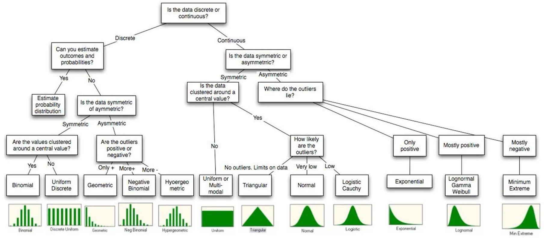
Last Updated: 2023-10-31