Table of Contents
Use This, Not That
R installation
Source
# Ubuntu 24.04
## Dependencies
sudo apt update
sudo apt build-dep r-base

## Specific R version
export R_VERSION=4.X.X

## Download and extract
curl -O https://cran.rstudio.com/src/base/R-4/R-${R_VERSION}.tar.gz
tar -xzvf R-${R_VERSION}.tar.gz
cd R-${R_VERSION}

## Build and install
./configure \
--prefix=/opt/R/${R_VERSION} \
--enable-memory-profiling \
--enable-R-shlib \
--with-blas \
--with-lapack

make
sudo make install

## Verify Install
/opt/R/${R_VERSION}/bin/R --version

## Create PATH symlinks to installation
sudo ln -s /opt/R/${R_VERSION}/bin/R /usr/local/bin/R
sudo ln -s /opt/R/${R_VERSION}/bin/Rscript /usr/local/bin/Rscript
Precompiled binaries
# Ubuntu 24.04
## Specific R version
export R_VERSION=4.X.X

## Download and install
curl -O https://cdn.posit.co/r/ubuntu-2404/pkgs/r-${R_VERSION}_1_$(dpkg --print-architecture).deb
sudo apt update
sudo apt install ./r-${R_VERSION}_1_$(dpkg --print-architecture).deb

## Verify Install
/opt/R/${R_VERSION}/bin/R --version

## Create PATH symlinks to installation
sudo ln -s /opt/R/${R_VERSION}/bin/R /usr/local/bin/R
sudo ln -s /opt/R/${R_VERSION}/bin/Rscript /usr/local/bin/Rscript

## Uninstall
#sudo rm -rf /opt/R/${R_VERSION}/
rig - RStudio’s R installation manager
# Ubuntu 22.04
## Download and install
`which sudo` curl -L https://rig.r-pkg.org/deb/rig.gpg -o /etc/apt/trusted.gpg.d/rig.gpg
`which sudo` sh -c 'echo "deb http://rig.r-pkg.org/deb rig main" > /etc/apt/sources.list.d/rig.list'
`which sudo` apt update
`which sudo` apt install r-rig

## Install R
rig add release
Packages
Software/Packages that make everyday tasks easier. Want to install all of them at once? See here https://bitbucket.org/bklamer/r-package-install/
Package management
- Dependency management
- renv
- RStudio’s dependency management, creates a ‘local’ library for project-based workflow
- Integrates with
rspm
- groundhog
- Dependency management, overloads the system library for script-based workflow
- rspm
- The Posit package manager provides URLs for installing archived snapshots of CRAN.
- Integrates with
renv, e.g.rspm::renv_init
- renv
- Package installation
- Package creation
Data IO
- readxl
- Import excel files
- readr
- Alternative functions for importing/exporting flat files
- tidyxl
- Import complex excel files and pass to unpivotr
- unpivotr
- Manipulate complex excel files into a data frame
- fst
- Fast serialization of objects
- fst vs. qs: Defaults to faster timing but larger sizes
- qs
- Fast serialization of objects
- qs vs. fst: Defaults to slower timing but smaller sizes
- data.table
- Fast functions for importing/exporting flat files
Data manipulation
- dplyr
- Data frame manipulation
- tidyr
- Data frame manipulation
- data.table
- Fast data frame manipulation
- tidytable
- data.table with dplyr/tidyr syntax
- janitor
- Data frame cleaning and preparation
Statistical computing
- matrixStats
- Fast matrix operations
- collapse
- Fast matrix and data frame operations
- ivs
- Manipulation of interval vectors
- slider
- Rolling window statistics
- Suitable for equally spaced time data
- roll
- Rolling window statistics
- Suitable for equally spaced time data
- runner
- Rolling window statistics
- Suitable for unequally spaced time data
Modeling
- Frameworks
- rms
- Harrellverse
- tidymodels
- Tidyverse
- mlr3
- Hyperparameter…verse?
- rms
- Mixed models
- Bayesian models
- Survival
- survival
- The original survival package
- coxme
- The original mixed-effects survival package
- cmprsk
- Competing risk models and their cumulative incidence
- tidycmprsk
cmprskhelpers
- survival
- Misc
- brglm2
- Firth’s bias reduced logistic model
- This package is preferred over logistf since
emmeanshas methods for it.
- betareg
- Beta regression
- ordbetareg
- Alternative to standard beta regression
- Generalized modeling of bounded outcomes
- See also https://github.com/glmmTMB/glmmTMB/tree/ordbetareg
- fixest
- Fast OLS and GLM regression
- MASS
- The original misc-model package
- VGAM
- Does almost everything linear/additive models
- quantreg
- Quantile regression
- afex
- linear and generalized linear mixed-effects models for design of experiments
- ordinal
- Ordinal models
- brglm2
- Generalized estimating equations
- Generalized additive models
- mgcv
- The original generalized additive modeling package
- gamm4
- gamm4 is based on gamm from package mgcv, but uses lme4 rather than nlme as the underlying fitting engine
- gam
- Trevor Hastie’s package, probably want to use mgcv instead
- gamlss
- Generalized additive model location, scale, and shape
- VGAM
- Does almost everything linear/additive models
- mgcv
- Time series
- Survey models
- SEM
- lavaan
- Most general SEM package
- lavaan
- Model helpers
- marginaleffects
- Marginal effects and adjusted predictions from statistical models
- emmeans
- Marginal effects and adjusted predictions from statistical models
- ggeffects
- Marginal effects and adjusted predictions from statistical models
- modelbased
- Marginal effects and adjusted predictions from statistical models
- pbkrtest
- F-tests for mixed-effects models (mainly lme4)
- glmglrt
- Generate likelihood ratio test p-values for model results in replacement of the usual Wald p-values. This also helps to match the profile likelihood confidence intervals.
- broom
- Summarize model results
- broom.mixed
- Summarize mixed-effects model results
- insight
- Summarize model results
- parameters
- Process model parameters
- performance
- Measure model performance
- equatiomatic
- Convert model objects into symbolic equations
- See also
rms::latex
- simputation
- A single interface to commonly used single imputation methods
- tidybayes
- Compose, extract, manipulate, and visualize posterior draws from Bayesian models
- bayestestR
- Describe posterior distributions from Bayesian models
- projpred
- Projection predictive feature selection for Bayesian models
- bayesplot
- Plotting functions for posterior analysis, MCMC diagnostics, prior and posterior predictive checks
- marginaleffects
Visualization
- Plotting
- Helpers
- scales
- Convert data scales/units for plot breaks or legends
- patchwork
- Combine and compose multiple ggplots
- ggbeeswarm
- Convert a 1d cloud of points into 2d cloud of points
- ggeffects
- Automatic average partial effect plots
- emmeans
- Automatic average partial effect plots
- modelbased
- Automatic average partial effect plots
- marginaleffects
- Automatic average partial effect plots
- modelsummary
- Automatic coefficient plots
- ggrepel
- Create non-overlapping labels
- ggpmisc
- Helpers for publication ready images (p-values…)
- ggsurvfit
- Survival and Kaplan-Meier plots
- visR
- Survival and Kaplan-Meier plots
- visdat
- Preliminary exploratory data visualisations of an entire dataset
- daggity
- Tools for analyzing DAGs
- ggdag
- Plot DAGs using ggplot2
- Gmisc
- Tools for plotting and tables
- scales
Tables
- gtsummary
- Automatic summary and regression HTML table generator
- flextable
- Manual table generation into HTML, Powerpoint, and Word
- huxtable
- Manual table generation into LaTeX
- gt
- Manual table generation into HTML
- sjPlot
- Automatic regression HTML table generator
- modelsummary
- Automatic regression table generation into HTML, LaTeX, Word, and Markdown
- kableExtra
- Build complex HTML or LaTeX tables using kable() from knitr
- texreg
- Automatic regression LaTeX table generator
Strings
- stringi
- Comprehensive string package
- stringr
- Simpler package built on stringi
- stringdist
- Approximate string matching
Dates and times
Report generation
- knitr
- The original Sweave replacement
- rmarkdown
- The original LaTeX replacement
- quarto
- The original rmarkdown replacement?
- litedown
- The new knitr and pandoc replacement
- report
- Automatic description of analyses
- tinytex
- Functions to install and maintain a lightweight, cross-platform, portable, and easy-to-maintain version of ‘TeX Live’
- minidown
- Minimal, responsive, and style-agnostic HTML documents with the lightweight CSS frameworks
Web tools
- blogdown
- Write blog posts and web pages in R Markdown
- shiny
- Build interactive web applications
- shinydashboard
- Create dashboards with Shiny
Misc
- microbenchmark
- Benchmark and analyze code execution times
- bench
- Benchmark and analyze code execution times
Project directory
Directory templates for starting a new consulting project.
Functions
First create some utility functions and data for the benchmarks below
library(ggplot2)
library(microbenchmark)
library(knitr)
set.seed(20171130)

#-------------------------------------------------------------------------------
# Check for equality of results in a microbenchmark run
#-------------------------------------------------------------------------------
check_equality <- function(values) {
  all(sapply(values[-1], function(x) identical(values[[1]], x)))
}

#-------------------------------------------------------------------------------
# Convert multiple microbenchmark runs into a summarized data.frame.
#-------------------------------------------------------------------------------
## data_list A named list of data that is used in func_list.
## func_list An alist object of functions to be tested.
## size A vector of integers that represent the data size.
## times An integer of the number of microbenchmark runs.
## unit A character for time units of the microbenchmark runs.
## check TRUE or FALSE whether or not to verify output is identical in the
## microbenchmark run.
mb_summary <- function(data_list, func_list, size, times = 30, unit = "s", check = TRUE) {
  # Check arguments
  list2env(data_list, envir = environment())

  if(check) {
    check <- function(values) {
      all(sapply(values[-1], function(x) identical(values[[1]], x)))
    }
  } else {
    check <- NULL
  }

  # Run benchmarks
  mb_results <- lapply(seq_along(size), function(x) {
    microbenchmark::microbenchmark(
      list = func_list,
      times = times,
      unit = unit,
      check = check
    )
  })

  # Create summary data.frame
  summary_results <- do.call(
    "rbind",
    lapply(seq_along(mb_results), function(x) {
      data.frame(
        size = size[x],
        summary(mb_results[[x]])
      )
    })
  )

  # return
  summary_results[c("size", "expr", "lq", "median", "uq", "neval")]
}

#-------------------------------------------------------------------------------
# Time conversions relative to 1 second (fractions of a second)
#-------------------------------------------------------------------------------
time_conversion <- function(time) {
  time_table <- data.frame(
    value = c(120, 60, 1, 10^-(1:9)),
    name = c(
      "min",
      rep("sec", each = 2),
      rep("ms", each = 3),
      rep("us", each = 3),
      rep("ns", each = 3)
    ),
    conversion = c(
      1/60,
      rep(1, 2),
      rep(1000, 3),
      rep(10^6, 3),
      rep(10^9, 3)
    ),
    stringsAsFactors = FALSE
  )
  closest_val = function(x,y){
    diff = y - x
    diff[diff <= 0] = NA
    if(all(is.na(diff))) {
      NA
    } else {
      which.min(diff)
    }
  }
  units <- time_table$name[sapply(time, closest_val, time_table$value)]
  convert <- time_table$conversion[sapply(time, closest_val, time_table$value)]
  paste(signif(time*convert, 3), units)
}

#-------------------------------------------------------------------------------
# Create a vector for the log scale times that will look "pretty" on the y-axis.
#-------------------------------------------------------------------------------
## df A data.frame as returned by mb_summary().
## n_ticks An integer as the suggestion for the number of tick marks.
log_breaks <- function(df, n_ticks = 5) {
  grDevices::axisTicks(
    usr = log(range(df$median, na.rm = TRUE), 10),
    log = TRUE,
    nint = n_ticks
  )
}

#-------------------------------------------------------------------------------
# Determine the units of a microbenchmark.
#-------------------------------------------------------------------------------
mb_units <- function(mb) {
  unit <- attr(mb, "unit")
  if(is.null(unit)) {
    attr(
      microbenchmark:::convert_to_unit(
        mb$time,
        sprintf("%ss", microbenchmark:::find_prefix(
          mb$time * 1e-09,
          minexp = -9,
          maxexp = 0,
          mu = FALSE))),
      "unit"
    )
  } else {
    unit
  }
}
== – Comparisons with missing values (NA)
This is based on the discussion at stackoverflow. I’ve summarized some of those results and elsewhere below.
The == function provides element by element equality comparison. However, as documented in ?"==",
Missing values (NA) and NaN values are regarded as non-comparable even to themselves, so comparisons involving them will always result in NA.
But sometimes it would be nice to have c(1, 2) == c(1, NA) evaluate to c(TRUE, FALSE) instead of c(TRUE, NA).
# These functions return TRUE wherever elements are the same, including NA's,
# and false everywhere else.
## Force element by element evaluation and returns. fun1 is for strict equality
## and fun2 will handle floating point numbers.
fun1 <- function(x, y) {
  mapply(identical, x, y)
}
fun2 <- function(x, y) {
  mapply(FUN = function(x, y) {isTRUE(all.equal(x, y))}, x, y)
}
## Modify results from ==
fun3 <- function(x, y) {
  eq <- (x == y)  |  (is.na(x) & is.na(y))
  eq[is.na(eq)] <- FALSE
  eq
}
fun4 <- function(x, y) {
  (is.na(x) & is.na(y)) | (!is.na(eq <- x == y) & eq)
}
fun5 <- function(x, y) {
  eq <- x == y
  na_eq <- which(is.na(eq))
  eq[na_eq] <- is.na(x[na_eq]) & is.na(y[na_eq])
  eq
}

# Check they result as we expect
x <- c(1, 2, 3)
y <- c(1, 2, 4)
res <- list(
  fun1(x, y),
  fun2(x, y),
  fun3(x, y),
  fun4(x, y),
  fun5(x, y)
)
check_equality(res)
## [1] TRUEx <- c(1, NA, 3)
y <- c(1, NA, 4)
res <- list(
fun1(x, y),
fun2(x, y),
fun3(x, y),
fun4(x, y),
fun5(x, y)
)
check_equality(res)## [1] TRUEx <- c(1, NA, 3)
y <- c(1, 2, 4)
res <- list(
fun1(x, y),
fun2(x, y),
fun3(x, y),
fun4(x, y),
fun5(x, y)
)
check_equality(res)## [1] TRUEx <- c(1, 2, 3)
y <- c(1, NA, 4)
res <- list(
fun1(x, y),
fun2(x, y),
fun3(x, y),
fun4(x, y),
fun5(x, y)
)
check_equality(res)## [1] TRUENow we’ll explore benchmarking and throw in the == case to see how slow our new functions are in comparison to it.
# Simulate data
vec_sizes <- 10^(1:4)
test_list <- lapply(vec_sizes, function(x) {
  list(
    x = sample(c(1:4, NA), size = x, replace = TRUE),
    y = sample(c(1:4, NA), size = x, replace = TRUE)
  )
})
test_functions <- alist(
  fun1 = fun1(test_list[[x]]$x, test_list[[x]]$y),
  fun2 = fun2(test_list[[x]]$x, test_list[[x]]$y),
  fun3 = fun3(test_list[[x]]$x, test_list[[x]]$y),
  fun4 = fun4(test_list[[x]]$x, test_list[[x]]$y),
  fun5 = fun5(test_list[[x]]$x, test_list[[x]]$y),
  `==` = test_list[[x]]$x == test_list[[x]]$y
)

# Run benchmark
res <- mb_summary(
  data_list = list(test_list = test_list),
  func_list  = test_functions,
  size = vec_sizes,
  times = 30,
  unit = "s",
  check = FALSE
)

# Plot results
ggplot(data = res, mapping = aes(x = size, y = median, color = expr)) +
  geom_line() +
  geom_point() +
  geom_pointrange(aes(ymin = lq, ymax = uq, color = expr), show.legend = FALSE) +
  scale_x_continuous(trans = "log10", breaks = vec_sizes, labels = vec_sizes) +
  scale_y_continuous(trans = "log10", breaks = log_breaks(res), labels = time_conversion(log_breaks(res))) +
  labs(
    title = "Comparing vectors with missing values (NA)",
    x = "Length of Vector",
    y = "Median Time",
    caption = "Both axis are on the log10 scale. \nPoint ranges (if visible) represent lower and upper quartiles."
  ) +
  annotation_logticks() +
  theme_bw()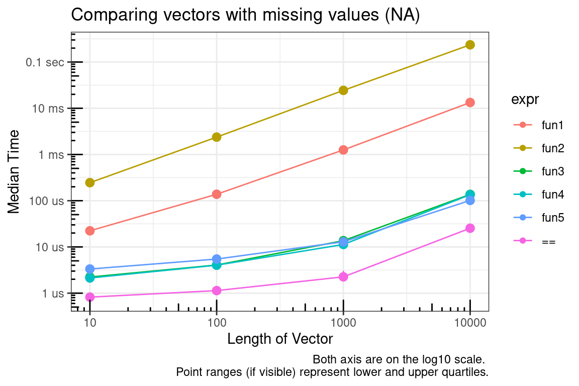
You can see that looping element by element comparisons is very slow (which is to be expected in R), but modifying the output from == is acceptable.
[ – Subsetting with logical and integer vectors
Subsetting with integer vectors is faster than logical vectors.
# Simulate data
vec_sizes <- 10^(1:6)
test_list <- lapply(vec_sizes, function(x) {
    sample(10L, size = x, replace = TRUE)
})
test_list_log <- lapply(test_list, function(x) {x > 5})
test_list_int <- lapply(test_list, function(x) {which(x > 5)})
test_functions <- alist(
  logical = test_list[[x]][test_list_log[[x]]],
  integer = test_list[[x]][test_list_int[[x]]]
)

# Run benchmark
res <- mb_summary(
  data_list = list(
    "test_list" = test_list,
    "test_list_log" = test_list_log,
    "test_list_int" = test_list_int
  ),
  func_list  = test_functions,
  size = vec_sizes,
  times = 30,
  unit = "s",
  check = TRUE
)

# Plot results
ggplot(data = res, mapping = aes(x = size, y = median, color = expr)) +
  geom_line() +
  geom_point() +
  geom_pointrange(aes(ymin = lq, ymax = uq, color = expr), show.legend = FALSE) +
  scale_x_continuous(trans = "log10", breaks = vec_sizes, labels = vec_sizes) +
  scale_y_continuous(trans = "log10", breaks = log_breaks(res), labels = time_conversion(log_breaks(res))) +
  labs(
    title = "Subsetting a vector (~50% dropped)",
    x = "Length of Vector",
    y = "Median Time",
    caption = "Both axis are on the log10 scale. \nPoint ranges (if visible) represent lower and upper quartiles."
  ) +
  annotation_logticks() +
  theme_bw()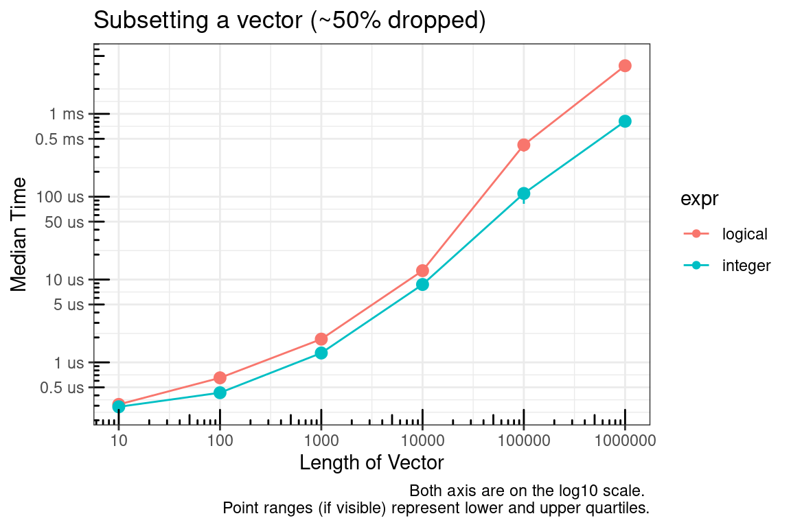
The logical vector, by definition, must be the same size as the vector to be subsetted and the integer vector can be much smaller. The plot above is for the case where approximately 50% of the vector is being subsetted (dropped). We’ll check this again for approximately 10% and 90%.
# Simulate data for 10% dropped
test_list_log <- lapply(test_list, function(x) {x > 1})
test_list_int <- lapply(test_list, function(x) {which(x > 1)})

# Run benchmark
res <- mb_summary(
  data_list = list(
    "test_list" = test_list,
    "test_list_log" = test_list_log,
    "test_list_int" = test_list_int
  ),
  func_list  = test_functions,
  size = vec_sizes,
  times = 30,
  unit = "s",
  check = TRUE
)

# Plot results
ggplot(data = res, mapping = aes(x = size, y = median, color = expr)) +
  geom_line() +
  geom_point() +
  geom_pointrange(aes(ymin = lq, ymax = uq, color = expr), show.legend = FALSE) +
  scale_x_continuous(trans = "log10", breaks = vec_sizes, labels = vec_sizes) +
  scale_y_continuous(trans = "log10", breaks = log_breaks(res), labels = time_conversion(log_breaks(res))) +
  labs(
    title = "Subsetting a vector (~10% dropped)",
    x = "Length of Vector",
    y = "Median Time",
    caption = "Both axis are on the log10 scale. \nPoint ranges (if visible) represent lower and upper quartiles."
  ) +
  annotation_logticks() +
  theme_bw()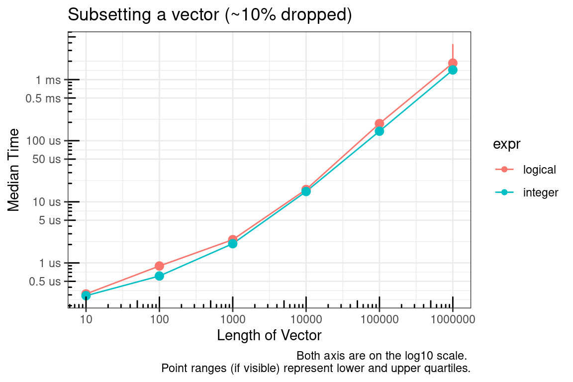
# Simulate data for 90% dropped
test_list_log <- lapply(test_list, function(x) {x > 9})
test_list_int <- lapply(test_list, function(x) {which(x > 9)})

# Run benchmark
res <- mb_summary(
  data_list = list(
    "test_list" = test_list,
    "test_list_log" = test_list_log,
    "test_list_int" = test_list_int
  ),
  func_list  = test_functions,
  size = vec_sizes,
  times = 30,
  unit = "s",
  check = TRUE
)

# Plot results
ggplot(data = res, mapping = aes(x = size, y = median, color = expr)) +
  geom_line() +
  geom_point() +
  geom_pointrange(aes(ymin = lq, ymax = uq, color = expr), show.legend = FALSE) +
  scale_x_continuous(trans = "log10", breaks = vec_sizes, labels = vec_sizes) +
  scale_y_continuous(trans = "log10", breaks = log_breaks(res), labels = time_conversion(log_breaks(res))) +
  labs(
    title = "Subsetting a vector (~90% dropped)",
    x = "Length of Vector",
    y = "Median Time",
    caption = "Both axis are on the log10 scale. \nPoint ranges (if visible) represent lower and upper quartiles."
  ) +
  annotation_logticks() +
  theme_bw()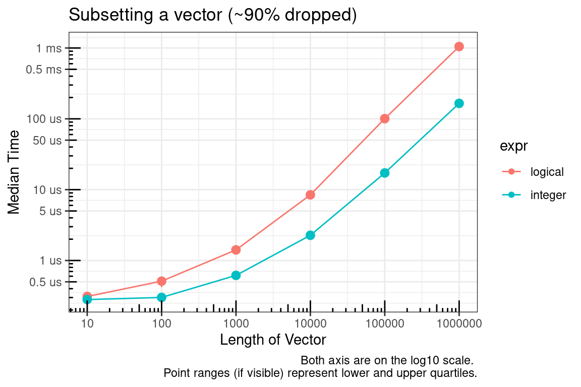
So it appears the main culprit is the size of the vector used to subset. Since an integer vector will often be smaller than a logical vector, using integers seems to be the logical choice :).
Next, you might say what about which? The time to convert the logical vector to integer was not considered in the previous benchmarks. As seen below, this is a valid concern.
# Simulate data for 10% dropped
test_list_log <- lapply(test_list, function(x) {x > 1})
test_list_int <- lapply(test_list, function(x) {which(x > 1)})
test_functions <- alist(
  logical = test_list[[x]][test_list_log[[x]]],
  `which(logical)` = test_list[[x]][which(test_list_log[[x]])]
)

# Run benchmark
res <- mb_summary(
  data_list = list(
    "test_list" = test_list,
    "test_list_log" = test_list_log,
    "test_list_int" = test_list_int
  ),
  func_list  = test_functions,
  size = vec_sizes,
  times = 30,
  unit = "s",
  check = TRUE
)

# Plot results
ggplot(data = res, mapping = aes(x = size, y = median, color = expr)) +
  geom_line() +
  geom_point() +
  geom_pointrange(aes(ymin = lq, ymax = uq, color = expr), show.legend = FALSE) +
  scale_x_continuous(trans = "log10", breaks = vec_sizes, labels = vec_sizes) +
  scale_y_continuous(trans = "log10", breaks = log_breaks(res), labels = time_conversion(log_breaks(res))) +
  labs(
    title = "Subsetting a vector (~10% dropped)",
    x = "Length of Vector",
    y = "Median Time",
    caption = "Both axis are on the log10 scale. \nPoint ranges (if visible) represent lower and upper quartiles."
  ) +
  annotation_logticks() +
  theme_bw()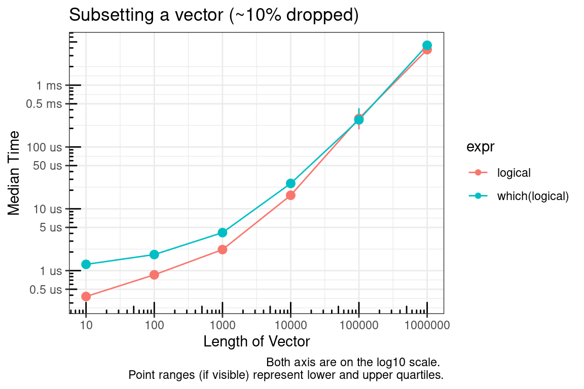
# Simulate data for 90% dropped
test_list_log <- lapply(test_list, function(x) {x > 9})
test_list_int <- lapply(test_list, function(x) {which(x > 9)})
test_functions <- alist(
  logical = test_list[[x]][test_list_log[[x]]],
  `which(logical)` = test_list[[x]][which(test_list_log[[x]])]
)

# Run benchmark
res <- mb_summary(
  data_list = list(
    "test_list" = test_list,
    "test_list_log" = test_list_log,
    "test_list_int" = test_list_int
  ),
  func_list  = test_functions,
  size = vec_sizes,
  times = 30,
  unit = "s",
  check = TRUE
)

# Plot results
ggplot(data = res, mapping = aes(x = size, y = median, color = expr)) +
  geom_line() +
  geom_point() +
  geom_pointrange(aes(ymin = lq, ymax = uq, color = expr), show.legend = FALSE) +
  scale_x_continuous(trans = "log10", breaks = vec_sizes, labels = vec_sizes) +
  scale_y_continuous(trans = "log10", breaks = log_breaks(res), labels = time_conversion(log_breaks(res))) +
  labs(
    title = "Subsetting a vector (~90% dropped)",
    x = "Length of Vector",
    y = "Median Time",
    caption = "Both axis are on the log10 scale. \nPoint ranges (if visible) represent lower and upper quartiles."
  ) +
  annotation_logticks() +
  theme_bw()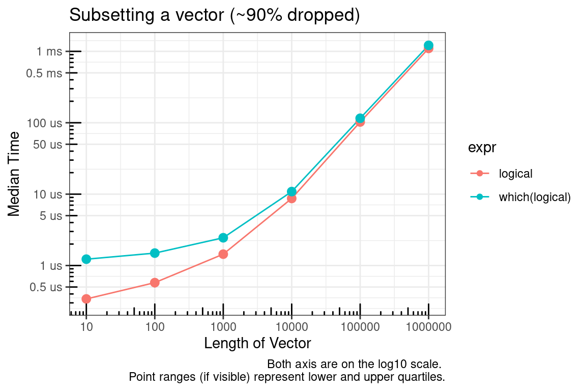
In summary, if you are able to pre-allocate the subset indices, then use integers. If you cannot pre-allocate then sticking with logical indices may make sense.
as.numeric – Convert a factor that is actually numeric
This comes straight from the ?factor documentation.
To transform a factor f to approximately its original numeric values, as.numeric(levels(f))[f] is recommended and slightly more efficient than as.numeric(as.character(f)).
We are only concerned about non-integer cases because as.integer handles factors as you would expect. If you need to convert numeric values or handle both cases (integer or numeric) then the two solutions to this problem are as.numeric(as.character(f)), which is usually easy to remember, and as.numeric(levels(f))[f], which is hard to remember. One interesting note is that the R FAQ provides a slightly different “hard” solution (as.numeric(levels(f))[as.integer(f)]) than found in the factor documentation.
The relative speed between these functions depends on the number of values in the levels of the factor. The ‘hard’ methods will convert a factor with a small number of levels faster than the easy method. If the number of levels is the same as the size of the factor, then all methods will be similar in speed.
These methods only work if the factor vector has levels/labels that are numeric.
# Simulate data
vec_sizes <- 10^(1:6)
## Make sure NA are handled correctly below
test_list <- lapply(vec_sizes, function(x) {
  factor(sample(c(rnorm(9), NA), x, replace = TRUE))
})
test_functions <- alist(
  hard_faq = as.numeric(levels(test_list[[x]]))[as.integer(test_list[[x]])],
  hard_doc = as.numeric(levels(test_list[[x]]))[test_list[[x]]],
  easy_doc = as.numeric(as.character(test_list[[x]]))
)

# Run benchmark
res <- mb_summary(
  data_list = list("test_list" = test_list),
  func_list  = test_functions,
  size = vec_sizes,
  times = 30,
  unit = "s",
  check = TRUE
)

# Plot results
ggplot(data = res, mapping = aes(x = size, y = median, color = expr)) +
  geom_line() +
  geom_point() +
  geom_pointrange(aes(ymin = lq, ymax = uq, color = expr), show.legend = FALSE) +
  scale_x_continuous(trans = "log10", breaks = vec_sizes, labels = vec_sizes) +
  scale_y_continuous(trans = "log10", breaks = log_breaks(res), labels = time_conversion(log_breaks(res))) +
  labs(
    title = "Converting a factor that is actually numeric (Level length ~9)",
    x = "Length of factor vector",
    y = "Median Time",
    caption = "Both axis are on the log10 scale. \nPoint ranges (if visible) represent lower and upper quartiles."
  ) +
  annotation_logticks() +
  theme_bw()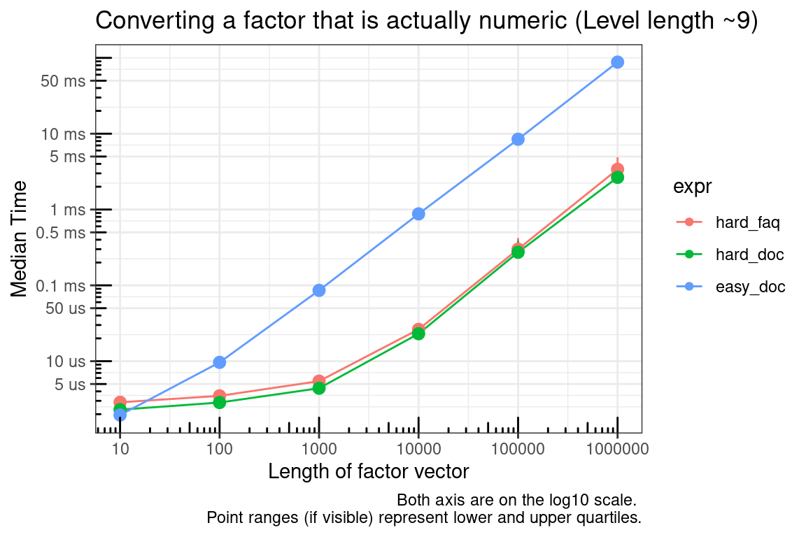
# Simulate data
vec_sizes <- 10^(1:6)
## Make sure NA are handled correctly below
test_list <- lapply(vec_sizes, function(x) {
  factor(c(rnorm(x), NA))
})
test_functions <- alist(
  hard_faq = as.numeric(levels(test_list[[x]]))[as.integer(test_list[[x]])],
  hard_doc = as.numeric(levels(test_list[[x]]))[test_list[[x]]],
  easy_doc = as.numeric(as.character(test_list[[x]]))
)

# Run benchmark
res <- mb_summary(
  data_list = list("test_list" = test_list),
  func_list  = test_functions,
  size = vec_sizes,
  times = 30,
  unit = "s",
  check = TRUE
)

# Plot results
ggplot(data = res, mapping = aes(x = size, y = median, color = expr)) +
  geom_line() +
  geom_point() +
  geom_pointrange(aes(ymin = lq, ymax = uq, color = expr), show.legend = FALSE) +
  scale_x_continuous(trans = "log10", breaks = vec_sizes, labels = vec_sizes) +
  scale_y_continuous(trans = "log10", breaks = log_breaks(res), labels = time_conversion(log_breaks(res))) +
  labs(
    title = "Converting a factor that is actually numeric (Level length ~N)",
    x = "Length of factor vector",
    y = "Median Time",
    caption = "Both axis are on the log10 scale. \nPoint ranges (if visible) represent lower and upper quartiles."
  ) +
  annotation_logticks() +
  theme_bw()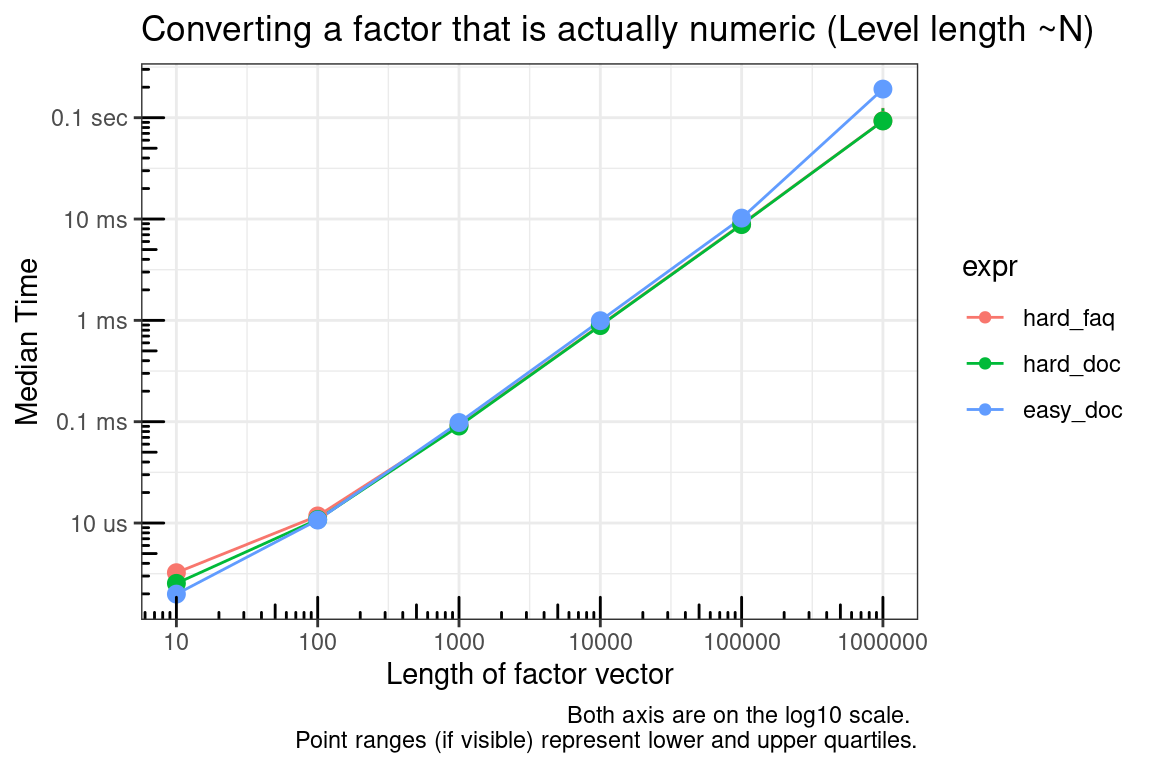
as.integer is the only choice that makes sense if you have strictly integer levels.
f <- factor(sample(1:9, 100, replace = TRUE))
mb <- summary(
  microbenchmark(
    as.integer = as.integer(f),
    hard_faq = as.integer(levels(f))[as.integer(f)],
    hard_doc = as.integer(levels(f))[f],
    easy_doc = as.integer(as.character(f)),
    check = check_equality
  ),
  unit = "relative"
)

tab <- mb[c("expr", "lq", "median", "uq", "neval")]
ftab <- flextable::flextable(data = tab)
ftab <- flextable::set_caption(x = ftab, caption = paste("Unit:", mb_units(mb)))
ftab <- flextable::colformat_double(x = ftab, digits = 1)
ftabexpr | lq | median | uq | neval |
as.integer | 1.0 | 1.0 | 1.0 | 100.0 |
hard_faq | 4.8 | 4.6 | 4.3 | 100.0 |
hard_doc | 3.8 | 3.6 | 3.4 | 100.0 |
easy_doc | 11.0 | 10.3 | 9.4 | 100.0 |
lengths – Get lengths along a list
length is a fast primitive function, but when finding the length of many objects along a list, lengths (notice the ending s) is better than applying length over the list.
# Simulate data
vec_sizes <- 10^(1:5)
test_list <- lapply(vec_sizes, function(x) {
  replicate(
    x,
    sample(10L, size = sample(10L, 1), replace = TRUE),
    simplify = FALSE
  )
})
test_functions <- alist(
  lengths = lengths(test_list[[x]]),
  vapply = vapply(
    X = test_list[[x]],
    FUN = length,
    FUN.VALUE = integer(1),
    USE.NAMES = FALSE
  )
)

# Run benchmark
res <- mb_summary(
  data_list = list("test_list" = test_list),
  func_list  = test_functions,
  size = vec_sizes,
  times = 30,
  unit = "s",
  check = TRUE
)

# Plot results
ggplot(data = res, mapping = aes(x = size, y = median, color = expr)) +
  geom_line() +
  geom_point() +
  geom_pointrange(aes(ymin = lq, ymax = uq, color = expr), show.legend = FALSE) +
  scale_x_continuous(trans = "log10", breaks = vec_sizes, labels = vec_sizes) +
  scale_y_continuous(trans = "log10", breaks = log_breaks(res), labels = time_conversion(log_breaks(res))) +
  labs(
    title = "Returning the length of list items",
    x = "Length of List",
    y = "Median Time",
    caption = "Both axis are on the log10 scale. \nPoint ranges (if visible) represent lower and upper quartiles."
  ) +
  annotation_logticks() +
  theme_bw()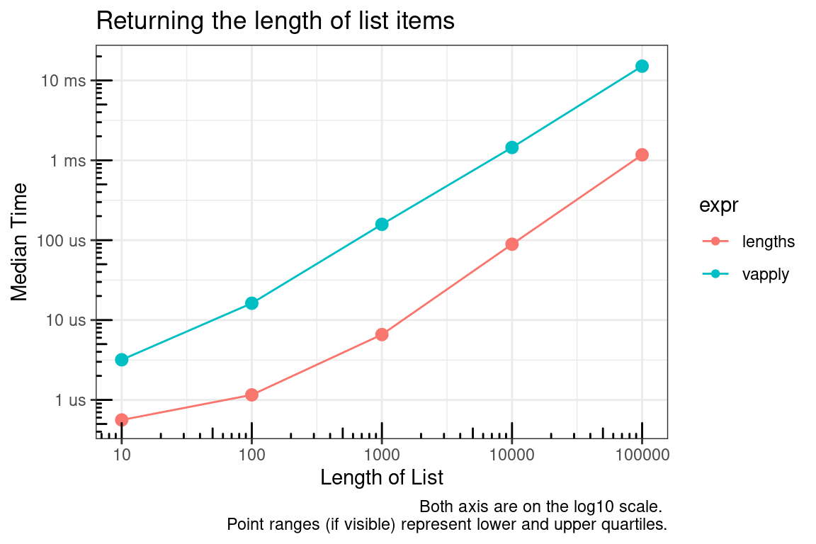
Microbenchmark summary for lengths of 1 and 100000.
mb1 <- microbenchmark(
  lengths = lengths(list(1)),
  vapply = vapply(
    X = list(1),
    FUN = length,
    FUN.VALUE = integer(1),
    USE.NAMES = FALSE
  ),
  times = 30,
  check = check_equality
)

tab <- summary(mb1)[c("expr", "lq", "median", "uq", "neval")]
ftab <- flextable::flextable(data = tab)
ftab <- flextable::set_caption(x = ftab, caption = paste("Unit:", mb_units(mb1)))
ftab <- flextable::colformat_double(x = ftab, digits = 0)
ftabexpr | lq | median | uq | neval |
lengths | 390 | 426 | 471 | 30 |
vapply | 1,643 | 1,674 | 1,743 | 30 |
mb2 <- microbenchmark(
  lengths = lengths(test_list[[length(vec_sizes)]]),
  vapply = vapply(
    X = test_list[[length(vec_sizes)]],
    FUN = length,
    FUN.VALUE = integer(1),
    USE.NAMES = FALSE
  ),
  times = 30,
  check = check_equality
)

tab <- summary(mb2)[c("expr", "lq", "median", "uq", "neval")]
ftab <- flextable::flextable(data = tab)
ftab <- flextable::set_caption(x = ftab, caption = paste("Unit:", mb_units(mb2)))
ftab <- flextable::colformat_double(x = ftab, digits = 0)
ftabexpr | lq | median | uq | neval |
lengths | 592 | 613 | 737 | 30 |
vapply | 13,723 | 13,885 | 14,666 | 30 |
nrow – Get data.frame row lengths
Here we compare the methods of getting the number of rows in a data.frame. Consider the penalty for cases of applying the function many times versus storing and calling the saved object.
- stored_value: The time it takes to get the length which has already been assigned to an object.
- stored_subset1: The time it takes to get the length from the object returned by
dimusing single bracket ([) indexing. - stored_subset2: as above using double bracket (
[[) indexing. - internal: Using the internal function
.row_names_info. Note that although this is an internal function with a dot name, it does appear to be safe to use being that it is a generic exported function. - primitive: using the primitive function
dimalong with single bracket ([) indexing. - convenience: using the convenience function
nrow(which just callsdim()[1L]).
The benchmark below has values for the simplest possible case.
# Simulate test data
data <- data.frame(a = 1)
dims <- dim(data)
n_row <- dims[1L]

# Benchmark methods
mb <- microbenchmark(
  stored_value = n_row,
  stored_subset1 = dims[1L],
  stored_subset2 = dims[[1L]],
  internal = .row_names_info(data, type = 2L),
  primitive = dim(data)[1L],
  convenience = nrow(data)
)

tab <- summary(mb)[c("expr", "lq", "median", "uq", "neval")]
ftab <- flextable::flextable(data = tab)
ftab <- flextable::set_caption(x = ftab, caption = paste("Unit:", mb_units(mb)))
ftab <- flextable::colformat_double(x = ftab, digits = 0)
ftabexpr | lq | median | uq | neval |
stored_value | 20 | 30 | 40 | 100 |
stored_subset1 | 60 | 70 | 90 | 100 |
stored_subset2 | 90 | 110 | 130 | 100 |
internal | 360 | 371 | 391 | 100 |
primitive | 1,493 | 1,523 | 1,603 | 100 |
convenience | 1,613 | 1,654 | 1,713 | 100 |
The following graph provides a summary of actually applying these methods to a list of dataframes.
# Simulate data
vec_sizes <- 10^(1:5)
## Note that the structure function below is just dput() output for
## data.frame(a=1), but is much faster for replicating.
test_list <- lapply(vec_sizes, function(x) {
  replicate(
    x,
    structure(list(a = 1), .Names = "a", row.names = c(NA, -1L), class = "data.frame"),
    simplify = FALSE
  )
})
test_functions <- alist(
  stored_subset1 = lapply(test_list[[x]], function(y) {dims[1]}),
  internal = lapply(test_list[[x]], function(y) {.row_names_info(y, type = 2L)}),
  primitive = lapply(test_list[[x]], function(y) {dim(y)[1L]}),
  convenience = lapply(test_list[[x]], function(y) {nrow(y)})
)

# Run benchmark
res <- mb_summary(
  data_list = list("test_list" = test_list),
  func_list  = test_functions,
  size = vec_sizes,
  times = 30,
  unit = "s",
  check = TRUE
)

# Plot results
ggplot(data = res, mapping = aes(x = size, y = median, color = expr)) +
  geom_line() +
  geom_point() +
  geom_pointrange(aes(ymin = lq, ymax = uq, color = expr), show.legend = FALSE) +
  scale_x_continuous(trans = "log10", breaks = vec_sizes, labels = vec_sizes) +
  scale_y_continuous(trans = "log10", breaks = log_breaks(res), labels = time_conversion(log_breaks(res))) +
  labs(
    title = "Returning number of rows in a data.frame",
    x = "Number of data.frames",
    y = "Median Time",
    caption = "Both axis are on the log10 scale. \nPoint ranges (if visible) represent lower and upper quartiles."
  ) +
  annotation_logticks() +
  theme_bw()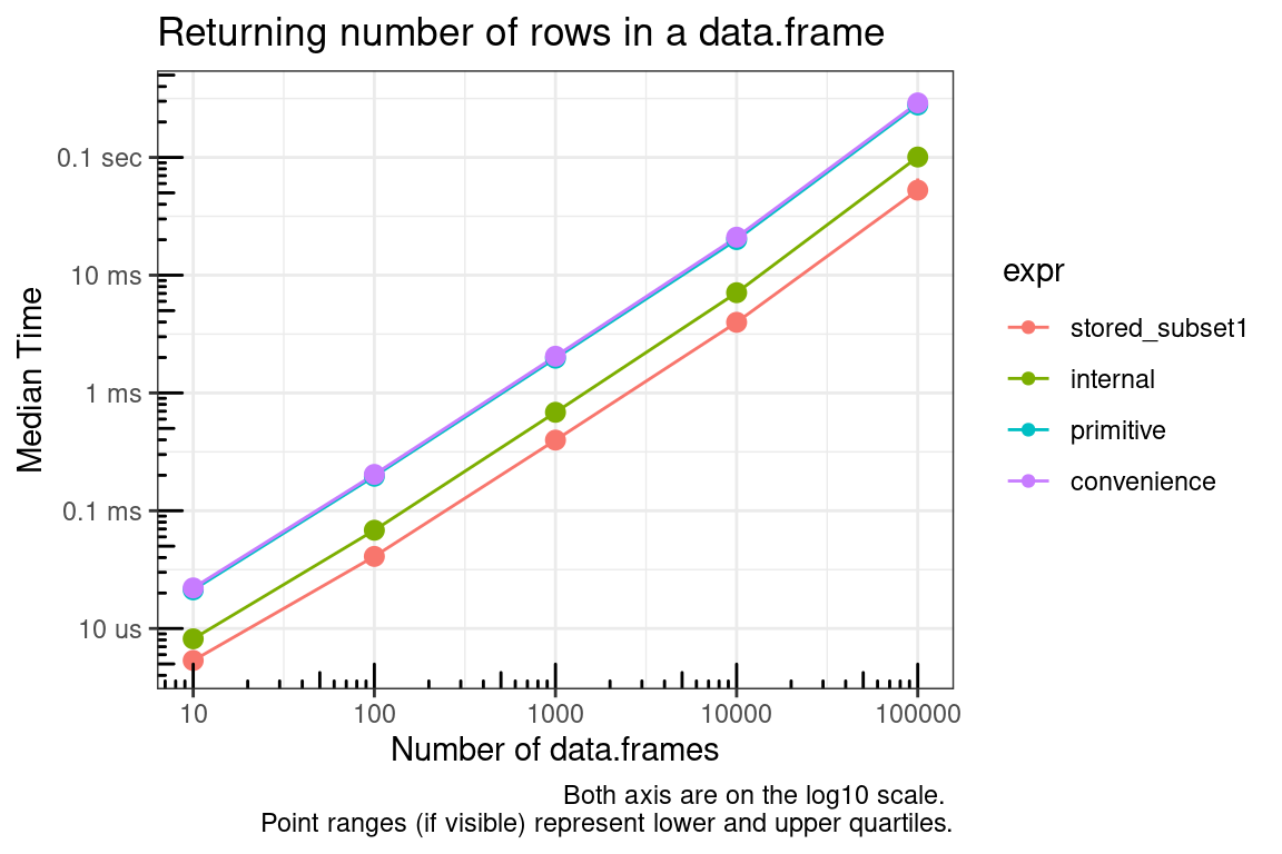
is.na, complete.cases, and is.finite – Subset immediately vs check then subset
When handling missing values and non-finite values, it it better to subset the data immediately, or should you first check the status and subset only if needed?
f_na1 <- function(x) {
  x
}

f_na2 <- function(x) {
  if(anyNA(x)) {
    x <- x[!is.na(x)]
  }
  x
}

f_na3 <- function(x) {
  x[!is.na(x)]
}

# Simulate data
vec_sizes <- 10^(1:5)
test_list <- lapply(vec_sizes, function(x) {rnorm(x)})
test_functions <- alist(
  f_na1 = lapply(test_list[[x]], function(y) f_na1(y)),
  f_na2 = lapply(test_list[[x]], function(y) f_na2(y)),
  f_na3 = lapply(test_list[[x]], function(y) f_na3(y))
)

# Run benchmark
res <- mb_summary(
  data_list = list(test_list = test_list),
  func_list = test_functions,
  size = vec_sizes,
  times = 30,
  unit = "s",
  check = FALSE
)

# Plot results
ggplot(data = res, mapping = aes(x = size, y = median, color = expr)) +
  geom_line() +
  geom_point() +
  geom_pointrange(aes(ymin = lq, ymax = uq, color = expr), show.legend = FALSE) +
  scale_x_continuous(trans = "log10", breaks = vec_sizes, labels = vec_sizes) +
  scale_y_continuous(trans = "log10", breaks = log_breaks(res), labels = time_conversion(log_breaks(res))) +
  labs(
    title = "is.na() Subset immediately vs check then subset",
    x = "Length of Vector",
    y = "Median Time",
    caption = "Both axis are on the log10 scale. \nPoint ranges (if visible) represent lower and upper quartiles."
  ) +
  annotation_logticks() +
  theme_bw()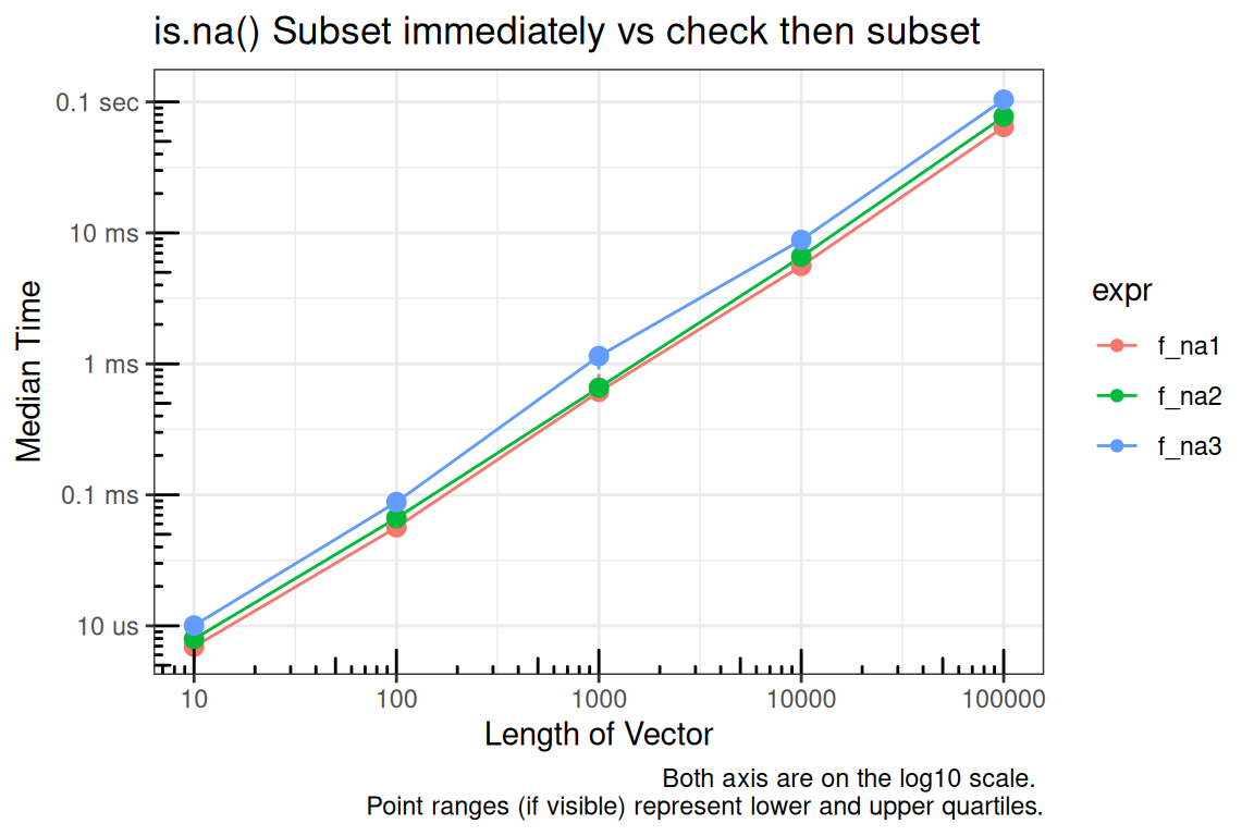
f_finite1 <- function(x) {
  x
}

f_finite2 <- function(x) {
  if(any(!is.finite(x))) {
    x <- x[is.finite(x)]
  }
  x
}

f_finite3 <- function(x) {
  x[is.finite(x)]
}

# Simulate data
vec_sizes <- 10^(1:5)
test_list <- lapply(vec_sizes, function(x) {rnorm(x)})
test_functions <- alist(
  f_finite1 = lapply(test_list[[x]], function(y) f_finite1(y)),
  f_finite2 = lapply(test_list[[x]], function(y) f_finite2(y)),
  f_finite3 = lapply(test_list[[x]], function(y) f_finite3(y))
)

# Run benchmark
res <- mb_summary(
  data_list = list(test_list = test_list),
  func_list  = test_functions,
  size = vec_sizes,
  times = 30,
  unit = "s",
  check = FALSE
)

# Plot results
ggplot(data = res, mapping = aes(x = size, y = median, color = expr)) +
  geom_line() +
  geom_point() +
  geom_pointrange(aes(ymin = lq, ymax = uq, color = expr), show.legend = FALSE) +
  scale_x_continuous(trans = "log10", breaks = vec_sizes, labels = vec_sizes) +
  scale_y_continuous(trans = "log10", breaks = log_breaks(res), labels = time_conversion(log_breaks(res))) +
  labs(
    title = "is.finite() Subset immediately vs check then subset",
    x = "Length of Vector",
    y = "Median Time",
    caption = "Both axis are on the log10 scale. \nPoint ranges (if visible) represent lower and upper quartiles."
  ) +
  annotation_logticks() +
  theme_bw()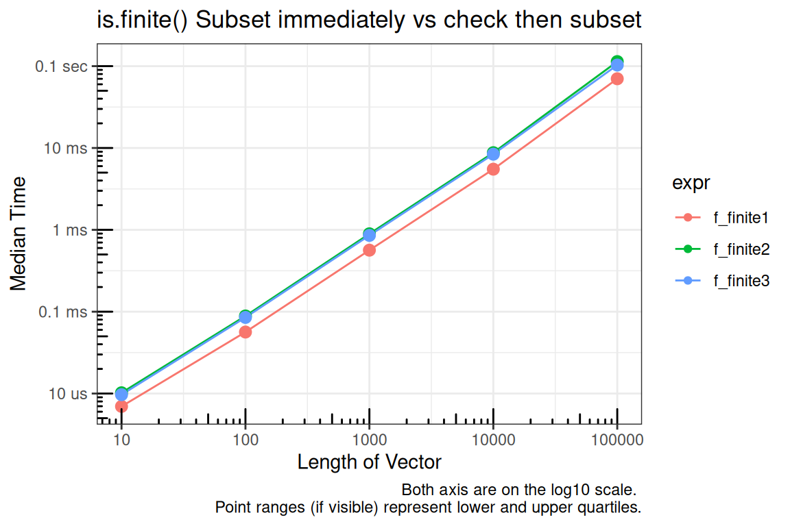
f_cc1 <- function(x) {
  list(x[[1L]], x[[2L]])
}

f_cc2 <- function(x) {
  if(anyNA(x[[1L]]) || anyNA(x[[2L]])) {
    ok <- complete.cases(x[[1L]], x[[2L]])
    x <- list(x[[1L]][ok], x[[2L]][ok])
  }
  x
}

f_cc3 <- function(x) {
  ok <- complete.cases(x[[1L]], x[[2L]])
  list(x[[1L]][ok], x[[2L]][ok])
}

# Simulate data
vec_sizes <- 10^(1:4)
test_list <- lapply(vec_sizes, function(x) {list(rnorm(x), rnorm(x))})
test_functions <- alist(
  f_cc1 = lapply(test_list[x], function(y) f_cc1(y)),
  f_cc2 = lapply(test_list[x], function(y) f_cc2(y)),
  f_cc3 = lapply(test_list[x], function(y) f_cc3(y))
)

# Run benchmark
res <- mb_summary(
  data_list = list(test_list = test_list),
  func_list = test_functions,
  size = vec_sizes,
  times = 30,
  unit = "s",
  check = FALSE
)

# Plot results
ggplot(data = res, mapping = aes(x = size, y = median, color = expr)) +
  geom_line() +
  geom_point() +
  geom_pointrange(aes(ymin = lq, ymax = uq, color = expr), show.legend = FALSE) +
  scale_x_continuous(trans = "log10", breaks = vec_sizes, labels = vec_sizes) +
  scale_y_continuous(trans = "log10", breaks = log_breaks(res), labels = time_conversion(log_breaks(res))) +
  labs(
    title = "complete.cases() Subset immediately vs check then subset",
    x = "Length of Vector",
    y = "Median Time",
    caption = "Both axis are on the log10 scale. \nPoint ranges (if visible) represent lower and upper quartiles."
  ) +
  annotation_logticks() +
  theme_bw()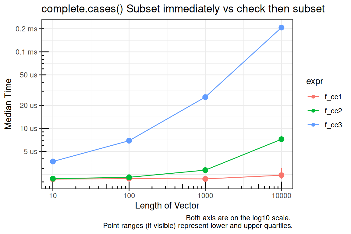
f_isna1 <- function(x) {
  if(anyNA(x[[1L]]) || anyNA(x[[2L]])) {
    ok <- !is.na(x[[1L]]) & !is.na(x[[2L]])
    x <- list(x[[1L]][ok], x[[2L]][ok])
  }
  x
}

f_isna2 <- function(x) {
  ok <- !is.na(x[[1L]]) & !is.na(x[[2L]])
  list(x[[1L]][ok], x[[2L]][ok])
}

f_cc3 <- function(x) {
  if(anyNA(x[[1L]]) || anyNA(x[[2L]])) {
    ok <- complete.cases(x[[1L]], x[[2L]])
    x <- list(x[[1L]][ok], x[[2L]][ok])
  }
  x
}

f_cc4 <- function(x) {
  ok <- complete.cases(x[[1L]], x[[2L]])
  list(x[[1L]][ok], x[[2L]][ok])
}

# Simulate data
vec_sizes <- 10^(1:4)
test_list <- lapply(vec_sizes, function(x) {list(c(rnorm(x)), c(rnorm(x)))})
test_functions <- alist(
  f_isna1 = lapply(test_list[x], function(y) f_isna1(y)),
  f_isna2 = lapply(test_list[x], function(y) f_isna2(y)),
  f_cc3 = lapply(test_list[x], function(y) f_cc3(y)),
  f_cc4 = lapply(test_list[x], function(y) f_cc4(y))
)

# Run benchmark
res <- mb_summary(
  data_list = list(test_list = test_list),
  func_list = test_functions,
  size = vec_sizes,
  times = 30,
  unit = "s",
  check = FALSE
)

# Plot results
ggplot(data = res, mapping = aes(x = size, y = median, color = expr)) +
  geom_line() +
  geom_point() +
  geom_pointrange(aes(ymin = lq, ymax = uq, color = expr), show.legend = FALSE) +
  scale_x_continuous(trans = "log10", breaks = vec_sizes, labels = vec_sizes) +
  scale_y_continuous(trans = "log10", breaks = log_breaks(res), labels = time_conversion(log_breaks(res))) +
  labs(
    title = "complete.cases() vs is.na()",
    x = "Length of Vector",
    y = "Median Time",
    caption = "Both axis are on the log10 scale. \nPoint ranges (if visible) represent lower and upper quartiles."
  ) +
  annotation_logticks() +
  theme_bw()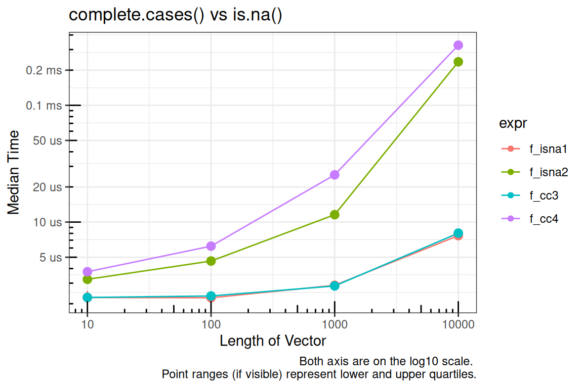
Last Updated: 2025-11-16