Variable Selection

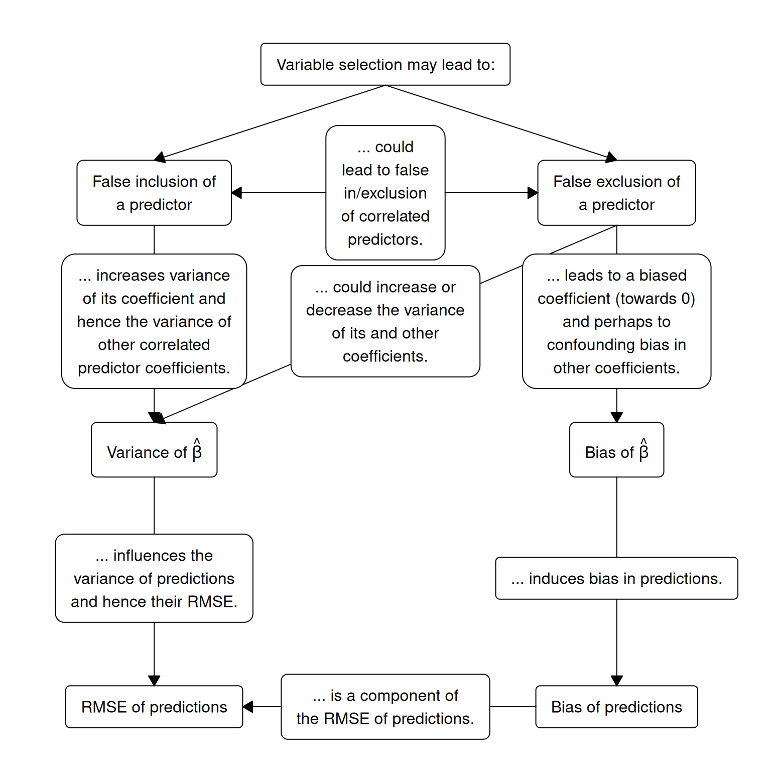
Miller (2002) provides a perspective using the traditional statistical approach for the purpose of prediction. Unfortunately his gloomy outlook on this topic is likely unchanged, even after decades of other advances and machine learning research being added to the statistical literature. However, the lure of variable selection is too great, so we should at least be aware its consequences. Heinze, Wallisch, and Dunkler (2018) provide a nice summary adapted in the following diagram:

Prediction models

Variable selection can be conducted using external methods or as intrinsically built into the learning method. John, Kohavi, and Pfleger (1994) referred to the external methods as filters and wrappers. Filter methods generally assess each individual variable and it’s association with the outcome or for other seemingly important properties such as relative variance. Wrapper methods generally involve subset selection using the model of interest such as forward and backwards selection. In contrast to traditional linear models, tree-based models and L1 regularized models have methods for variable selection built into the model algorithm. Since statistical methods cannot distinguish between spurious and real associations, usually the best outcomes will be seen when subject matter expertise is used as a first step in the variable selection process.

Tree-based models
1. Use subject matter expertise, usually in combination with unsupervised learning, to select the relevant predictor variables.
2. Fit the model inside a cross-validitory framework to generate internally validated predictive performance estimates.
L1 regularized linear models
1. Use subject matter expertise, usually in combination with unsupervised learning, to select the relevant predictor variables.
2. Use subject matter expertise and model exploration to determine appropriate functional form. If unsure where to start, try comparing model performance to an intrinsic method which is nonlinear in nature. This may help elucidate the decision process. Ideally this process would be packaged in an algorithm to be included in cross validation, though often this step is only feasible using manual intervention.
3. Fit the model inside a cross-validitory framework to generate internally validated predictive performance estimates.
Linear models or models without intrinsic variable selection
1. Use subject matter expertise, usually in combination with unsupervised learning, to select the relevant predictor variables.
2. Use subject matter expertise and model exploration to determine appropriate functional form. If unsure where to start, try comparing model performance from intrinsic methods which are linear and nonlinear in nature. This may help elucidate the decision process. Ideally this process would be packaged in an algorithm to be included in cross validation, though often this step is only feasible using manual intervention.
3. Fit the model inside a cross-validitory framework to generate predictive performance estimates. Incorporate the filter or wrapper method within the resampling process.

The benefits of intrinsic variable selection are ease, speed, and efficiency (direct connection between variable selection and the objective function). However, this comes at the cost of dependency on learning method and tuning parameters. If using external variable selection, it is critical to include this step within the resampling process of model validation.

Unsupervised learning

Unsupervised learning is used to estimate relationships between potential predictor variables without the use of a response variable. Common methods include principal components analysis (PCA) and clustering. These methods are used for the general goal of data reduction, providing more incite when working with a large number of parameters.

PCA is useful when we wish to generate derived variables and visualize relationships within the data. PCA creates uncorrelated linear combinations of the \(p\) predictors which explain the maximal amount of variation in the data. Each principal component is a normalized linear combination of each predictor, where the predictors are weighted by loadings, the sum of the squared loadings are equal to 1, and the linear predictor itself is the score of the principal component. Thus, the principal component score vectors have length N and the principal component loading vector has length \(p\). The principal component loading is found through optimization by eigen decomposition. By constraining the second principal component to be uncorrelated with the first, we have a nice geometric result that the second principal component is orthogonal to the first. Loading vectors can be visualized for each variable considered (usually in two dimensional space of the first and second principal components) which may inform which variables contain the same or differing information. Before PCA is conducted, numeric variables should be centered to have mean zero, and if measured on different units, scaled to have standard deviation of 1. Scree plots are commonly used to determine the optimal number of principle components. This is an ad hoc technique which tries to determine the point at which the proportion of variance explained by each subsequent principal component drops off (where it begins to level off).

Variable clustering is used to partition variables into distinct groups so that variables within each group are similar and variables in different groups are different. A common method of variable clustering is known as hierarchical clustering. Hierarchical clustering is advantageous compared to k-means clustering because pre-specification of the number of cluster k is not required and the resulting dendrogram allows us to easily insert our own preconceived beliefs :). Cluster groups in hierarchical clustering are defined by cutting the dendrogram horizontally and grouping variables using the lines which were cut through. To form the dendrogram, you may use an agglomerative method (variables start individually and are pairs are merged up the hierarchy; bottom-up) or divisive method (variables start together and are split down the hierarchy; top-down). A measure dissimilarity is needed. Common options are Euclidean distance (linear and monotonic relationships), squared Euclidean distance, Hoeffding’s D (can capture a wide variety of relationships), Spearman’s \(\rho\) (monotonic relationships), or Gower’s distance (can be used with categorical variables). Finally, dissimilarity between 2 groups of variables are determined by their linkage. Linkage can be defined as complete (maximal (pairwise) intercluster dissimilarity), single (minimal (pairwise) intercluster dissimilarity), average (mean (pairwise) intercluster dissimilarity), and centroid (dissimilarity between group 1 and group 2’s centroid). Average and complete linkage methods are the most common. Generally best results are obtained when variables are standardized (centered and scaled) before hierarchical clustering takes place. To check robustness of results, try performing hierarchical clustering on a subset of the data or with different methods choices and see if results match.

Finally, you may wish to remove variables which are highly correlated or redundant with each other. Gregorich et al. (2021) provides a nice overview on how this may impact the analysis for the three major areas of modeling.

External variable selection

Filter methods usually assign a numeric score to each predictor or set of predictors. This allows us to rank the predictors (or sets) and use a cut-off to select which is included in the model. The following methods are commonly used to assign this score:

Categorical outcome
- Categorical predictors
  - Chi-squared test
  - Odds ratio (for 2-level predictor)
- Numeric predictors
  - t-test (for 2-level predictor)
  - F-test (for 3+ level predictor)
  - ROC-AUC
  - PR-AUC
Numeric outcome
- Categorical predictors
  - t-test (for 2-level predictor)
  - F-test (for 3+ level predictor)
  - ROC-AUC
  - PR-AUC
- Numeric predictors
  - Correlation (linear or monotonic relationships)
  - Mutual information (nonlinear relationships)

Alternatively, flexible multivariable models can test sets of predictors, using chunk tests for their combined importance, or model-free methods such as feature ordering by conditional independence (FOCI) by Azadkia and Chatterjee (2021).

Wrapper methods usually assess the performance of the model itself on differing sets of variables using a search algorithm. Common search algorithms include

Backward selection
- Not feasible if p > n
- aka recursive feature elimination (RFE), backward-stepwise elimination, etc.
Forward selection
- Not recommended
Hybrid backwards and forwards selection
Genetic algorithm
Simulated annealing

The algorithm for backward selection looks like:

For each variable subset size \(i = I, \dots, 1\)
1. Fit the model with the top \(i\) variables
2. Calculate the model predictive performance
3. Calculate each variable’s importance score and update the rankings for the next iteration.
Rank the performance estimates for each top subset \(i\)
Choose the optimal set of variables \(i\) to fit the final model.

External variable selection should always be embedded within a cross-validity framework. i.e. predictive performance is assessed on a hold-out/assessment/test set which is different than what was used to fit the model and assign variable importance. This ensures generalizability and assessment of robustness for the procedure.

Bootstrap resampling of the variable selection method may show if the data is capable of selecting a seemingly robust model. High inclusion frequency of the same variables would indicate a stable selection process, however, colinearity will obstruct this.

Bibliography

Azadkia, Mona, and Sourav Chatterjee. 2021. “A Simple Measure of Conditional Dependence.” https://arxiv.org/abs/1910.12327.

Gregorich, Mariella, Susanne Strohmaier, Daniela Dunkler, and Georg Heinze. 2021. “Regression with Highly Correlated Predictors: Variable Omission Is Not the Solution.” International Journal of Environmental Research and Public Health 18 (8): 4259. https://doi.org/10.3390/ijerph18084259.

Heinze, Georg, Christine Wallisch, and Daniela Dunkler. 2018. “Variable Selection - A Review and Recommendations for the Practicing Statistician.” Biometrical Journal 60 (3): 431–49. https://doi.org/10.1002/bimj.201700067.

John, George H., Ron Kohavi, and Karl Pfleger. 1994. “Irrelevant Features and the Subset Selection Problem.” In Machine Learning Proceedings 1994, 121–29. Elsevier. https://doi.org/10.1016/B978-1-55860-335-6.50023-4.

Miller, Alan. 2002. Subset Selection in Regression. 2nd ed. Chapman; Hall/CRC. https://doi.org/10.1201/9781420035933.

Published: 2022-02-16