Simulate BNB data

Simulate data from the bivariate negative binomial (BNB) distribution. The BNB distribution is used to simulate count data where the event counts are jointly dependent (correlated). For independent data, see sim_nb().

Usage

sim_bnb(
  n,
  mean1,
  mean2,
  ratio,
  dispersion,
  nsims = 1L,
  return_type = "list",
  max_zeros = 0.99
)

Arguments

n

(integer: [2, Inf))
The number(s) of paired observations.

mean1

(numeric: (0, Inf))
The mean(s) of sample 1 $(\mu_1)$.

mean2, ratio

(numeric: (0, Inf))
Only specify one of these arguments.

mean2: The mean(s) of sample 2 $(\mu_2)$.
ratio: The ratio(s) of means for sample 2 with respect to sample 1 $\left( r = \frac{\mu_2}{\mu_1} \right)$.

mean2 = ratio * mean1

dispersion

(numeric: (0, Inf))
The gamma distribution shape parameter(s) $(\theta)$ which control the dispersion and the correlation between sample 1 and 2. See 'Details' and 'Examples'.

nsims

(Scalar integer: 1L; [1, Inf))
The expected number of simulated data sets. If nsims > 1, the data is returned in a list-column of a depower simulation data frame. nsims may be reduced depending on max_zeros.

return_type

(string: "list"; c("list", "data.frame"))
The data structure of the simulated data. If "list" (default), a list object is returned. If "data.frame" a data frame in tall format is returned. The list object provides computational efficiency and the data frame object is convenient for formulas. See 'Value'.

max_zeros

(Scalar numeric: 0.99; [0, 1])
The maximum proportion of zeros each group in a simulated dataset is allowed to have. If the proportion of zeros is greater than this value, the corresponding data is excluded from the set of simulations. This is most likely to occur when the sample size is small and the dispersion parameter is small.

Value

If nsims = 1 and the number of unique parameter combinations is one, the following objects are returned:

If return_type = "list", a list:
Slot Name Description
1 Simulated counts from sample 1.
2 Simulated counts from sample 2.
If return_type = "data.frame", a data frame:
Column Name Description
1 item Subject/item indicator.
2 condition Sample/condition indicator.
3 value Simulated counts.

If nsims > 1 or the number of unique parameter combinations is greater than one, each object described above is returned in a list-column named data in a depower simulation data frame:

Column	Name	Description
1	`n1`	Sample size of sample 1.
2	`n2`	Sample size of sample 2.
3	`mean1`	Mean for sample 1.
4	`mean2`	Mean for sample 2.
5	`ratio`	Ratio of means (sample 2 / sample 1).
6	`dispersion`	Gamma distribution shape parameter (dispersion).
7	`nsims`	Number of valid simulation iterations.
8	`distribution`	Distribution sampled from.
9	`data`	List-column of simulated data.

Details

The negative binomial distribution may be defined using a gamma-Poisson mixture distribution. In this case, the Poisson parameter $\lambda$ is a random variable with gamma distribution. Equivalence between different parameterizations are demonstrated below:

# Define constants and their relationships
n <- 10000
dispersion <- 8
mu <- 4
p <- dispersion / (dispersion + mu)
q <- mu / (mu + dispersion)
variance <- mu + (mu^2 / dispersion)
rate <- p / (1 - p)
scale <- (1 - p) / p

# alternative formula for mu
mu_alt <- (dispersion * (1 - p)) / p
stopifnot(isTRUE(all.equal(mu, mu_alt)))

set.seed(20240321)

# Using built-in rnbinom with dispersion and mean
w <- rnbinom(n = n, size = dispersion, mu = mu)

# Using gamma-Poisson mixture with gamma rate parameter
x <- rpois(
  n = n,
  lambda = rgamma(n = n, shape = dispersion, rate = rate)
)

# Using gamma-Poisson mixture with gamma scale parameter
y <- rpois(
  n = n,
  lambda = rgamma(n = n, shape = dispersion, scale = scale)
)

# Using gamma-Poisson mixture with multiplicative mean and
# gamma scale parameter
z <- rpois(
  n = n,
  lambda = mu * rgamma(n = n, shape = dispersion, scale = 1/dispersion)
)

# Compare CDFs
par(mar=c(4,4,1,1))
plot(
  x = sort(w),
  y = (1:n)/n,
  xlim = range(c(w,x,y,z)),
  ylim = c(0,1),
  col = 'green',
  lwd = 4,
  type = 'l',
  main = 'CDF'
)
lines(x = sort(x), y = (1:n)/n, col = 'red', lwd = 2)
lines(x = sort(y), y = (1:n)/n, col = 'yellow', lwd = 1.5)
lines(x = sort(z), y = (1:n)/n, col = 'black')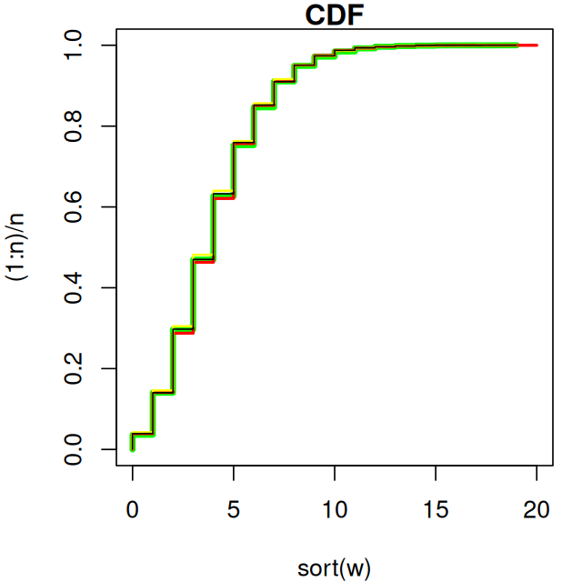

The BNB distribution is implemented by compounding two conditionally independent Poisson random variables $X_1 \mid G = g \sim \text{Poisson}(\mu g)$ and $X_2 \mid G = g \sim \text{Poisson}(r \mu g)$ with a gamma random variable $G \sim \text{Gamma}(\theta, \theta^{-1})$. The probability mass function for the joint distribution of $X_1, X_2$ is

$$ P(X_1 = x_1, X_2 = x_2) = \frac{\Gamma(x_1 + x_2 + \theta)}{(\mu + r \mu + \theta)^{x_1 + x_2 + \theta}} \frac{\mu^{x_1}}{x_1!} \frac{(r \mu)^{x_2}}{x_2!} \frac{\theta^{\theta}}{\Gamma(\theta)} $$

where $x_1,x_2 \in \mathbb{N}^{\geq 0}$ are specific values of the count outcomes, $\theta \in \mathbb{R}^{> 0}$ is the dispersion parameter which controls the dispersion and level of correlation between the two samples (otherwise known as the shape parameter of the gamma distribution), $\mu \in \mathbb{R}^{> 0}$ is the mean parameter, and $r = \frac{\mu_2}{\mu_1} \in \mathbb{R}^{> 0}$ is the ratio parameter representing the multiplicative change in the mean of the second sample relative to the first sample. $G$ denotes the random subject effect and the gamma distribution scale parameter is assumed to be the inverse of the dispersion parameter ($\theta^{-1}$) for identifiability.

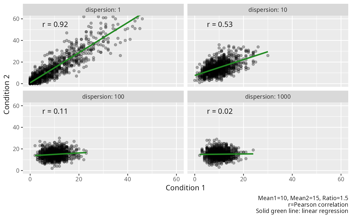
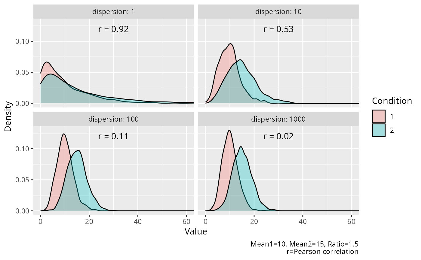
Correlation decreases from 1 to 0 as the dispersion parameter increases from 0 to infinity. For a given dispersion, increasing means also increases the correlation. See 'Examples' for a demonstration.

See 'Details' in sim_nb() for additional information on the negative binomial distribution.

References

Yu L, Fernandez S, Brock G (2020). “Power analysis for RNA-Seq differential expression studies using generalized linear mixed effects models.” BMC Bioinformatics, 21(1), 198. ISSN 1471-2105, doi:10.1186/s12859-020-3541-7 .

Rettiganti M, Nagaraja HN (2012). “Power Analyses for Negative Binomial Models with Application to Multiple Sclerosis Clinical Trials.” Journal of Biopharmaceutical Statistics, 22(2), 237–259. ISSN 1054-3406, 1520-5711, doi:10.1080/10543406.2010.528105 .

Aban IB, Cutter GR, Mavinga N (2009). “Inferences and power analysis concerning two negative binomial distributions with an application to MRI lesion counts data.” Computational Statistics & Data Analysis, 53(3), 820–833. ISSN 01679473, doi:10.1016/j.csda.2008.07.034 .

Examples

#----------------------------------------------------------------------------
# sim_bnb() examples
#----------------------------------------------------------------------------
library(depower)

# Paired two-sample data returned in a data frame
sim_bnb(
  n = 10,
  mean1 = 10,
  ratio = 1.6,
  dispersion = 3,
  nsims = 1,
  return_type = "data.frame"
)
#>    item condition value
#> 1     1         1     0
#> 2     2         1    23
#> 3     3         1     5
#> 4     4         1     1
#> 5     5         1    19
#> 6     6         1     4
#> 7     7         1     7
#> 8     8         1    13
#> 9     9         1    10
#> 10   10         1    11
#> 11    1         2     1
#> 12    2         2    40
#> 13    3         2     5
#> 14    4         2     7
#> 15    5         2    27
#> 16    6         2     7
#> 17    7         2     2
#> 18    8         2    36
#> 19    9         2    18
#> 20   10         2    17

# Paired two-sample data returned in a list
sim_bnb(
  n = 10,
  mean1 = 10,
  ratio = 1.6,
  dispersion = 3,
  nsims = 1,
  return_type = "list"
)
#> $value1
#>  [1] 10  4  5 14 15 14  4 23  5 19
#> 
#> $value2
#>  [1] 17  8  4 24 12 24 21 43 14 26
#> 

# Two simulations of paired two-sample data
# returned as a list of data frames
sim_bnb(
  n = 10,
  mean1 = 10,
  ratio = 1.6,
  dispersion = 3,
  nsims = 2,
  return_type = "data.frame"
)
#> # A tibble: 1 × 9
#>      n1    n2 mean1 mean2 ratio dispersion1 nsims distribution            data  
#>   <dbl> <dbl> <dbl> <dbl> <dbl>       <dbl> <dbl> <chr>                   <list>
#> 1    10    10    10    16   1.6           3     2 Dependent two-sample B… <list>

# Two simulations of Paired two-sample data
# returned as a list of lists
sim_bnb(
  n = 10,
  mean1 = 10,
  ratio = 1.6,
  dispersion = 3,
  nsims = 2,
  return_type = "list"
)
#> # A tibble: 1 × 9
#>      n1    n2 mean1 mean2 ratio dispersion1 nsims distribution            data  
#>   <dbl> <dbl> <dbl> <dbl> <dbl>       <dbl> <dbl> <chr>                   <list>
#> 1    10    10    10    16   1.6           3     2 Dependent two-sample B… <list>

#----------------------------------------------------------------------------
# Visualization of the BNB distribution as dispersion varies.
# The first figure shows the marginal distribution for each group.
# The second figure shows the joint distribution for each group.
#----------------------------------------------------------------------------
set.seed(1234)
data <- lapply(
  X = c(1, 10, 100, 1000),
  FUN = function(x) {
    d <- sim_bnb(
      n = 1000,
      mean1 = 10,
      ratio = 1.5,
      dispersion = x,
      nsims = 1,
      return_type = "data.frame"
    )
    cor <- cor(
      x = d[d$condition == "1", ]$value,
      y = d[d$condition == "2", ]$value
    )
    cbind(dispersion = x, correlation = cor, d)
  }
)

data <- do.call(what = "rbind", args = data)

# Density plot of marginal distributions
ggplot2::ggplot(
  data = data,
  mapping = ggplot2::aes(x = value, fill = condition)
) +
  ggplot2::facet_wrap(
    facets = ggplot2::vars(.data$dispersion),
    ncol = 2,
    labeller = ggplot2::labeller(.rows = ggplot2::label_both)
  ) +
  ggplot2::geom_density(alpha = 0.3) +
  ggplot2::coord_cartesian(xlim = c(0, 60)) +
  ggplot2::geom_text(
    mapping = ggplot2::aes(
      x = 30,
      y = 0.12,
      label = paste0("r = ", round(correlation, 2))
    ),
    check_overlap = TRUE
  ) +
  ggplot2::labs(
    x = "Value",
    y = "Density",
    fill = "Condition",
    caption = "Mean1=10, Mean2=15, Ratio=1.5\nr=Pearson correlation"
  )


# Reshape to wide format for scatterplot
data_wide <- data.frame(
  dispersion = data[data$condition == "1", ]$dispersion,
  correlation = data[data$condition == "1", ]$correlation,
  value1 = data[data$condition == "1", ]$value,
  value2 = data[data$condition == "2", ]$value
)

# Scatterplot of joint distribution
ggplot2::ggplot(
  data = data_wide,
  mapping = ggplot2::aes(x = value1, y = value2)
) +
  ggplot2::facet_wrap(
    facets = ggplot2::vars(.data$dispersion),
    ncol = 2,
    labeller = ggplot2::labeller(.rows = ggplot2::label_both)
  ) +
  ggplot2::geom_point(alpha = 0.3) +
  ggplot2::geom_smooth(
    method = "lm",
    se = FALSE,
    color = "forestgreen"
  ) +
  ggplot2::geom_text(
    data = unique(data_wide[c("dispersion", "correlation")]),
    mapping = ggplot2::aes(
      x = 5,
      y = 55,
      label = paste0("r = ", round(correlation, 2))
    ),
    hjust = 0
  ) +
  ggplot2::coord_cartesian(xlim = c(0, 60), ylim = c(0, 60)) +
  ggplot2::labs(
    x = "Condition 1",
    y = "Condition 2",
    caption = paste0(
      "Mean1=10, Mean2=15, Ratio=1.5",
      "\nr=Pearson correlation",
      "\nSolid green line: linear regression"
    )
  )
#> `geom_smooth()` using formula = 'y ~ x'

Slot	Name	Description
1		Simulated counts from sample 1.
2		Simulated counts from sample 2.