Simulate NB data

Simulate data from two independent negative binomial (NB) distributions. For paired data, see sim_bnb().

Usage

sim_nb(
  n1,
  n2 = n1,
  mean1,
  mean2,
  ratio,
  dispersion1,
  dispersion2 = dispersion1,
  nsims = 1L,
  return_type = "list",
  max_zeros = 0.99
)

Arguments

n1

(integer: [2, Inf))
The sample size(s) of group 1.

n2

(integer: n1; [2, Inf))
The sample size(s) of group 2.

mean1

(numeric: (0, Inf))
The mean(s) of group 1 $(\mu_1)$.

mean2, ratio

(numeric: (0, Inf))
Only specify one of these arguments.

mean2: The mean(s) of group 2 $(\mu_2)$.
ratio: The ratio(s) of means for group 2 with respect to group 1 $\left( r = \frac{\mu_2}{\mu_1} \right)$.

mean2 = ratio * mean1

dispersion1

(numeric: (0, Inf))
The dispersion parameter(s) of group 1 $(\theta_1)$. See 'Details' and 'Examples'.

dispersion2

(numeric: dispersion1; (0, Inf))
The dispersion parameter(s) of group 2 $(\theta_2)$. See 'Details' and 'Examples'.

nsims

(Scalar integer: 1L; [1,Inf))
The expected number of simulated data sets. If nsims > 1, the data is returned in a list-column of a depower simulation data frame. nsims may be reduced depending on max_zeros.

return_type

(string: "list"; c("list", "data.frame"))
The data structure of the simulated data. If "list" (default), a list object is returned. If "data.frame" a data frame in tall format is returned. The list object provides computational efficiency and the data frame object is convenient for formulas. See 'Value'.

max_zeros

(Scalar numeric: 0.99; [0, 1])
The maximum proportion of zeros each group in a simulated dataset is allowed to have. If the proportion of zeros is greater than this value, the corresponding data is excluded from the set of simulations. This is most likely to occur when the sample size is small and the dispersion parameter is small.

Value

If nsims = 1 and the number of unique parameter combinations is one, the following objects are returned:

If return_type = "list", a list:
Slot Name Description
1 value1 Simulated counts from group 1.
2 value2 Simulated counts from group 2.
If return_type = "data.frame", a data frame:
Column Name Description
1 item Subject/item indicator.
2 condition Group/condition indicator.
3 value Simulated counts.

If nsims > 1 or the number of unique parameter combinations is greater than one, each object described above is returned in a list-column named data in a depower simulation data frame:

Column	Name	Description
1	`n1`	Sample size of group 1.
2	`n2`	Sample size of group 2.
3	`mean1`	Mean for group 1.
4	`mean2`	Mean for group 2.
5	`ratio`	Ratio of means (group 2 / group 1).
6	`dispersion1`	Dispersion parameter for group 1.
7	`dispersion2`	Dispersion parameter for group 2.
8	`nsims`	Number of valid simulation iterations.
9	`distribution`	Distribution sampled from.
10	`data`	List-column of simulated data.

Details

The negative binomial distribution has many parameterizations. In the regression modeling context, it is common to specify the distribution in terms of its mean and dispersion. We use the following probability mass function:

$$ \begin{aligned} P(X = x) &= \dbinom{x + \theta - 1}{x} \left( \frac{\theta}{\theta + \mu} \right)^{\theta} \left( \frac{\mu}{\mu + \theta} \right)^x \\ &= \frac{\Gamma(x + \theta)}{x! \Gamma(\theta)} \left( \frac{\theta}{\theta + \mu} \right)^{\theta} \left( \frac{\mu}{\mu + \theta} \right)^{x} \\ &= \frac{\Gamma(x + \theta)}{(\theta + \mu)^{\theta + x}} \frac{\theta^{\theta}}{\Gamma(\theta)} \frac{\mu^{x}}{x!} \end{aligned} $$

where $x \in \mathbb{N}^{\geq 0}$, $\theta \in \mathbb{R}^{> 0}$ is the dispersion parameter, and $\mu \in \mathbb{R}^{> 0}$ is the mean. This is analogous to the typical formulation where $X$ is counting $x$ failures given $\theta$ successes and $p = \frac{\theta}{\theta + \mu}$ is the probability of success on each trial. It follows that $E(X) = \mu$ and $Var(X) = \mu + \frac{\mu^2}{\theta}$. The $\theta$ parameter describes the 'dispersion' among observations. Smaller values of $\theta$ lead to overdispersion and larger values of $\theta$ decrease the overdispersion, eventually converging to the Poisson distribution.

Described above is the 'indirect quadratic parameterization' of the negative binomial distribution, which is commonly found in the R ecosystem. However, it is somewhat counterintuitive because the smaller $\theta$ gets, the larger the overdispersion. The 'direct quadratic parameterization' of the negative binomial distribution may be found in some R packages and other languages such as SAS and Stata. The direct parameterization is defined by substituting $\alpha = \frac{1}{\theta}$ ($\alpha > 0$) which results in $Var(X) = \mu + \alpha\mu^2$. In this case, the larger $\alpha$ gets the larger the overdispersion, and the Poisson distribution is a special case of the negative binomial distribution where $\alpha = 0$.

A general class of negative binomial models may be defined with mean $\mu$ and variance $\mu + \alpha\mu^{p}$. The 'linear parameterization' is then found by setting $p=1$, resulting in $Var(X) = \mu + \alpha\mu$. It's common to label the linear parameterization as 'NB1' and the direct quadratic parameterization as 'NB2'.

See 'Details' in sim_bnb() for additional information on the gamma-Poisson mixture formulation of the negative binomial distribution.

References

Yu L, Fernandez S, Brock G (2017). “Power analysis for RNA-Seq differential expression studies.” BMC Bioinformatics, 18(1), 234. ISSN 1471-2105, doi:10.1186/s12859-017-1648-2 .

Rettiganti M, Nagaraja HN (2012). “Power Analyses for Negative Binomial Models with Application to Multiple Sclerosis Clinical Trials.” Journal of Biopharmaceutical Statistics, 22(2), 237–259. ISSN 1054-3406, 1520-5711, doi:10.1080/10543406.2010.528105 .

Aban IB, Cutter GR, Mavinga N (2009). “Inferences and power analysis concerning two negative binomial distributions with an application to MRI lesion counts data.” Computational Statistics & Data Analysis, 53(3), 820–833. ISSN 01679473, doi:10.1016/j.csda.2008.07.034 .

Hilbe JM (2011). Negative Binomial Regression, 2 edition. Cambridge University Press. ISBN 9780521198158 9780511973420, doi:10.1017/CBO9780511973420 .

Hilbe JM (2014). Modeling count data. Cambridge University Press, New York, NY. ISBN 9781107028333 9781107611252, doi:10.1017/CBO9781139236065 .

Cameron AC, Trivedi PK (2013). Regression Analysis of Count Data, Econometric Society Monographs, 2 edition. Cambridge University Press. doi:10.1017/CBO9781139013567 .

Examples

#----------------------------------------------------------------------------
# sim_nb() examples
#----------------------------------------------------------------------------
library(depower)

# Independent two-sample NB data returned in a data frame
sim_nb(
  n1 = 10,
  mean1 = 5,
  ratio = 1.6,
  dispersion1 = 0.5,
  dispersion2 = 0.5,
  nsims = 1,
  return_type = "data.frame"
)
#>    item condition value
#> 1     1         1     4
#> 2     2         1     0
#> 3     3         1     0
#> 4     4         1     0
#> 5     5         1     0
#> 6     6         1     9
#> 7     7         1     1
#> 8     8         1     0
#> 9     9         1     0
#> 10   10         1     5
#> 11    1         2     8
#> 12    2         2     3
#> 13    3         2     7
#> 14    4         2     0
#> 15    5         2    22
#> 16    6         2     0
#> 17    7         2    23
#> 18    8         2     4
#> 19    9         2     0
#> 20   10         2     2

# Independent two-sample NB data returned in a list
sim_nb(
  n1 = 10,
  mean1 = 5,
  ratio = 1.6,
  dispersion1 = 0.5,
  dispersion2 = 0.5,
  nsims = 1,
  return_type = "list"
)
#> $value1
#>  [1]  0  3  0  0 18  2  1  3  2  0
#> 
#> $value2
#>  [1] 94  8  6  3 10  0  1 42  3 74
#> 

# Two simulations of independent two-sample data
# returned as a list of data frames
sim_nb(
  n1 = 10,
  mean1 = 5,
  ratio = 1.6,
  dispersion1 = 0.5,
  dispersion2 = 0.5,
  nsims = 2,
  return_type = "data.frame"
)
#> # A tibble: 1 × 10
#>      n1    n2 mean1 mean2 ratio dispersion1 dispersion2 nsims distribution      
#>   <dbl> <dbl> <dbl> <dbl> <dbl>       <dbl>       <dbl> <dbl> <chr>             
#> 1    10    10     5     8   1.6         0.5         0.5     2 Independent two-s…
#> # ℹ 1 more variable: data <list>

# Two simulations of independent two-sample data
# returned as a list of lists
sim_nb(
  n1 = 10,
  mean1 = 5,
  ratio = 1.6,
  dispersion1 = 0.5,
  dispersion2 = 0.5,
  nsims = 2,
  return_type = "list"
)
#> # A tibble: 1 × 10
#>      n1    n2 mean1 mean2 ratio dispersion1 dispersion2 nsims distribution      
#>   <dbl> <dbl> <dbl> <dbl> <dbl>       <dbl>       <dbl> <dbl> <chr>             
#> 1    10    10     5     8   1.6         0.5         0.5     2 Independent two-s…
#> # ℹ 1 more variable: data <list>

#----------------------------------------------------------------------------
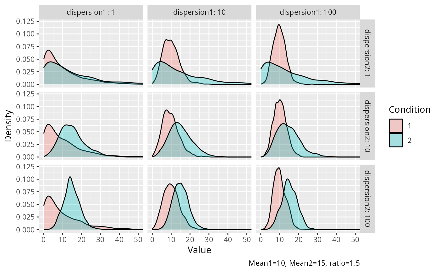
# Visualization of the NB distribution as dispersion varies between groups.
# Small dispersion values result in higher variance (overdispersed) and
# large dispersion values result in lower variance (converges to Poisson).
#----------------------------------------------------------------------------
disp <- expand.grid(c(1, 10, 100), c(1, 10, 100))
set.seed(1234)
data <- mapply(
  FUN = function(disp1, disp2) {
    d <- sim_nb(
      n1 = 1000,
      mean1 = 10,
      ratio = 1.5,
      dispersion1 = disp1,
      dispersion2 = disp2,
      nsims = 1,
      return_type = "data.frame"
    )
    cbind(dispersion1 = disp1, dispersion2 = disp2, d)
  },
  disp1 = disp[[1]],
  disp2 = disp[[2]],
  SIMPLIFY = FALSE
)

data <- do.call(what = "rbind", args = data)

ggplot2::ggplot(
  data = data,
  mapping = ggplot2::aes(x = value, fill = condition)
) +
  ggplot2::facet_grid(
    rows = ggplot2::vars(.data$dispersion2),
    cols = ggplot2::vars(.data$dispersion1),
    labeller = ggplot2::labeller(
      .rows = ggplot2::label_both,
      .cols = ggplot2::label_both
    )
  ) +
  ggplot2::geom_density(alpha = 0.3) +
  ggplot2::coord_cartesian(xlim = c(0, 50)) +
  ggplot2::labs(
    x = "Value",
    y = "Density",
    fill = "Condition",
    caption = "Mean1=10, Mean2=15, ratio=1.5"
  )

Slot	Name	Description
1	`value1`	Simulated counts from group 1.
2	`value2`	Simulated counts from group 2.