Partition a tree from build_tree() — cut

Cuts a tree produced by build_tree() into k clusters, recomputing for each cluster the weighted synthetic variable (first component score).

Usage

cut_tree(x, k, cor_matrix = FALSE)

Arguments

x: An object returned by build_tree().
k: (Scalar integer)
Desired number of clusters (1 <= k <= p).
cor_matrix: (Scalar logical: FALSE)
If TRUE, returns 1) squared association matrices among variables within each cluster and 2) squared correlation matrix for the synthetic variables.

Value

A list with elements:

scores: \(n \times k\) data frame of synthetic variables for each cluster (first principal component).
scores_cor_matrix: Pearson correlation matrix for the synthetic variables.
vars: A four-column data frame:
- cluster: Cluster membership
- variable: Variable names
- squared_association: If numeric, the weighted squared Pearson correlations \(r^2\) with the cluster PC1. If factor, the weighted squared correlations \(\eta^2(y\mid g)\) with the cluster PC1.
- association: If numeric, weighted Pearson correlation \(r\) with the cluster PC1. If factor, the weighted correlations \(\eta(x \mid g)\) with the cluster PC1.
vars_cor_matrix: List of squared association matrices among variables within each cluster. Similarity for numeric:numeric is squared Pearson's correlation \(r^2\); numeric:categorical is the correlation ratio \(\eta^2(y\mid g)\); categorical:categorical is the squared canonical correlation between their dummy sets.
cluster: Integer vector (length \(p\)) assigning each variable to a cluster.
H: Homogeneity for each cluster, defined as the sum of squared associations with the cluster's first principal component.
Hprop: Proportion of total homogeneity accounted for by the partition \(k\). The gain in cohesion. Defined as \(\frac{H(P_k) - H(P_1)}{H(P_p) - H(P_1)}\). Where \(P_k\) is the chosen cluster partition (K=k), \(P_1\) is a single cluster partition (K=1), and \(P_p\) is the singleton cluster partition (K=p).
size: Number of variables in each cluster.
k: The chosen number of clusters.
call: The matched call.
method: "cut_tree"

Examples

#----------------------------------------------------------------------------
# cut_tree() examples
#----------------------------------------------------------------------------
library(vclust)

# Example 1: Quantitative variables with equal weights
set.seed(42)
n <- 60
data <- data.frame(
  col1 = rnorm(n),
  col2 = rnorm(n),
  col3 = rnorm(n),
  col4 = rnorm(n),
  weights = rep(1, n)
)

tree <- build_tree(data = data, weights = "weights")
plot(tree)
rect.hclust(tree = tree, k = 2)

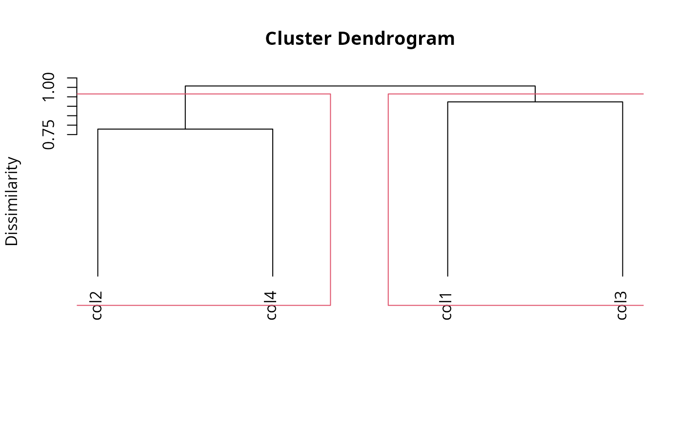cut <- cut_tree(tree, k = 2)
cut
#> $scores
#>      cluster_1   cluster_2
#> 1  -0.53092974 -1.96246847
#> 2   0.47814944 -0.74476264
#> 3   0.03875632 -0.02737220
#> 4   0.73519003 -1.10273815
#> 5  -0.47339012 -0.15534006
#> 6   1.94095621 -0.18462579
#> 7  -0.41401141 -1.33676229
#> 8   0.24939028 -1.48483985
#> 9   1.25019316 -2.14570794
#> 10  1.69014242  0.28078933
#> 11 -1.10032079 -0.25190794
#> 12  0.07543063 -1.71902001
#> 13  0.16259703  0.95682962
#> 14  0.14751063  1.17876341
#> 15  0.20482752  1.34540779
#> 16 -0.52530295 -1.18603597
#> 17  0.15667764  0.17756819
#> 18 -0.22441469  2.71513510
#> 19 -2.24295252  1.22764604
#> 20 -1.08469958 -0.76362776
#> 21  2.62726760  0.21671579
#> 22 -0.18643568  0.48082876
#> 23 -0.97683935 -0.15717899
#> 24 -1.83815455 -0.67967022
#> 25  0.02473929 -1.41256188
#> 26  1.25649205  1.26501438
#> 27  0.25985190 -0.13372343
#> 28  0.56033118  0.83774658
#> 29  1.11028825  0.37602086
#> 30  0.66146673 -0.36272684
#> 31  1.90474629 -0.21853121
#> 32 -2.09761978 -1.59679659
#> 33  0.29734797  0.40082152
#> 34  1.02610169  0.25204154
#> 35 -1.38152878 -0.59518647
#> 36 -0.82640344  0.15703501
#> 37 -0.90460405  0.57613228
#> 38 -2.42441091 -0.02465810
#> 39  0.10757060  1.15973300
#> 40  1.39295952  1.11718881
#> 41  0.50858099 -0.17323526
#> 42  0.96599497 -0.54798284
#> 43 -0.49807708 -0.24086303
#> 44  2.15623111  0.25282626
#> 45 -0.98224344  1.42194772
#> 46  0.09369090  0.98872647
#> 47 -0.86006709 -0.20498680
#> 48 -0.03667365 -0.42965318
#> 49  0.53892212  0.43253586
#> 50 -1.01488090  0.41585030
#> 51  0.06859869 -0.28898361
#> 52 -0.78598850  1.25970385
#> 53  0.44010207 -2.29296096
#> 54 -0.15250243  1.06680675
#> 55 -1.20976299  0.74141579
#> 56 -0.11646054 -0.19688680
#> 57 -1.58522159 -1.49791578
#> 58  2.00061033  0.56173611
#> 59 -1.38007028  2.34180995
#> 60  0.72225127 -0.08506598
#> 
#> $scores_cor_matrix
#> NULL
#> 
#> $vars
#>   cluster variable squared_association association
#> 1       1     col2           0.6104559   0.7813167
#> 2       1     col4           0.6104559  -0.7813167
#> 3       2     col3           0.5384371   0.7337827
#> 4       2     col1           0.5384371  -0.7337827
#> 
#> $vars_cor_matrix
#> $vars_cor_matrix$cluster_1
#> NULL
#> 
#> $vars_cor_matrix$cluster_2
#> NULL
#> 
#> 
#> $cluster
#> col1 col2 col3 col4 
#>    2    1    2    1 
#> 
#> $H
#> cluster_1 cluster_2 
#>  1.220912  1.076874 
#> 
#> $Hprop
#> [1] 0.3717936
#> 
#> $size
#> cluster_1 cluster_2 
#>         2         2 
#> 
#> $k
#> [1] 2
#> 
#> $call
#> cut_tree(x = tree, k = 2)
#> 
#> $method
#> [1] "cut_tree"
#> 

# Example 2: Mixed data with equal weights
set.seed(70)
n <- 80
data <- data.frame(
  col1 = rnorm(n),
  col2 = rnorm(n) + 0.6*rnorm(n),
  col3 = factor(sample(letters[1:3], n, TRUE)),
  col4 = factor(sample(c("L","M","H"), n, TRUE)),
  w = rep(1, n)
)

tree2 <- build_tree(data = data, weights = "w")
plot(tree2)
rect.hclust(tree = tree2, k = 2)

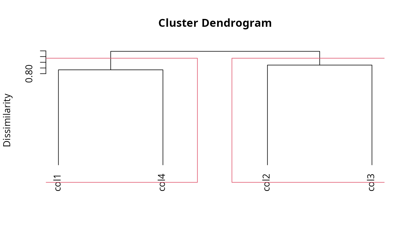cut2 <- cut_tree(tree2, k = 2)
cut2
#> $scores
#>      cluster_1   cluster_2
#> 1  -1.84182208 -0.82942427
#> 2   1.15519658 -0.20232127
#> 3   1.73280932  0.16982541
#> 4  -1.04106312 -0.27146976
#> 5   0.16862641  2.41923489
#> 6   0.78732026 -0.57634370
#> 7  -0.44665320  0.39418731
#> 8  -0.96917606  0.37941742
#> 9  -1.96057213 -2.03909106
#> 10  1.19165526 -0.55805262
#> 11  0.24903009 -1.27675641
#> 12 -0.04478659  2.27817568
#> 13 -0.53286870 -1.40944351
#> 14  1.88085909  0.01760342
#> 15  0.90282592  0.68843012
#> 16 -0.41942040  1.18296585
#> 17 -0.04892064  0.64857346
#> 18  0.48237678  0.20462019
#> 19  0.74597488  0.80429476
#> 20  0.37916895 -0.47395642
#> 21 -1.10251157 -1.01958231
#> 22 -0.75146486  1.36135440
#> 23 -0.72765687  1.05846511
#> 24 -0.40020921  0.77959274
#> 25 -0.49278440 -0.33389380
#> 26 -2.02482110 -0.85655409
#> 27 -0.56417898  0.22773742
#> 28 -1.19337132  0.78928087
#> 29  1.23946993 -0.35583502
#> 30  1.59049748 -1.60248604
#> 31  1.89725465  1.53122461
#> 32 -1.42407196 -1.34769226
#> 33  0.53637543  0.62344775
#> 34  0.74968551  0.49512270
#> 35 -0.74739005 -0.88405114
#> 36 -0.67111132 -1.46990319
#> 37 -1.07848712  1.79535162
#> 38 -0.10136184  0.39453819
#> 39 -0.84081452  0.41932388
#> 40  0.61574946 -0.46764972
#> 41 -0.47178997 -0.95028452
#> 42 -0.18052034 -0.09948218
#> 43  0.62400108  1.72972659
#> 44 -2.12003169 -0.47367017
#> 45 -0.80066654 -0.88676724
#> 46 -0.10950066 -0.16740953
#> 47  1.12344700 -0.45523437
#> 48 -0.12539556  1.12067228
#> 49 -0.35088646 -0.26351525
#> 50  0.93899815  2.08744514
#> 51 -0.06242523 -1.27231950
#> 52  1.19323995 -2.26002126
#> 53 -0.94095864 -1.80668021
#> 54 -1.29091054  1.52674595
#> 55  0.33218769 -0.01186647
#> 56  0.83425321 -0.80191127
#> 57  1.88505375  0.50672254
#> 58 -0.38005902  1.51191124
#> 59 -2.27766669  1.15553974
#> 60 -0.11344632 -0.37245014
#> 61 -0.60871716  0.16620519
#> 62  1.00835914 -1.81207174
#> 63  0.29850986  0.50040850
#> 64  0.66226314 -0.17507331
#> 65 -1.53784890  0.24065465
#> 66  1.00759276  0.99334702
#> 67  1.25707210 -0.07214911
#> 68  0.89334804  0.44641973
#> 69  0.37237397 -0.92242886
#> 70 -0.40391385 -0.88881362
#> 71  1.18601264 -0.99637899
#> 72 -1.10508243 -0.03047388
#> 73  3.09417267  1.92420482
#> 74 -1.37137803  0.22546214
#> 75 -0.80975891 -0.42804421
#> 76  1.72425255  1.46076668
#> 77  0.58320736 -1.73747392
#> 78 -1.10907128 -0.49451842
#> 79 -0.18507914  0.17653459
#> 80  0.45740434 -1.08198983
#> 
#> $scores_cor_matrix
#> NULL
#> 
#> $vars
#>   cluster variable squared_association association
#> 1       1     col1           0.5831399   0.7636360
#> 2       1     col4           0.5831399   0.7636360
#> 3       2     col2           0.5623250   0.7498833
#> 4       2     col3           0.5623250   0.7498833
#> 
#> $vars_cor_matrix
#> $vars_cor_matrix$cluster_1
#> NULL
#> 
#> $vars_cor_matrix$cluster_2
#> NULL
#> 
#> 
#> $cluster
#> col1 col2 col3 col4 
#>    1    2    2    1 
#> 
#> $H
#> cluster_1 cluster_2 
#>   1.16628   1.12465 
#> 
#> $Hprop
#> [1] 0.3681551
#> 
#> $size
#> cluster_1 cluster_2 
#>         2         2 
#> 
#> $k
#> [1] 2
#> 
#> $call
#> cut_tree(x = tree2, k = 2)
#> 
#> $method
#> [1] "cut_tree"
#> 

# Example 3: Mixed data with unequal weights
data$w <- rexp(n)

tree3 <- build_tree(data = data, weights = "w")
plot(tree3)
rect.hclust(tree = tree3, k = 2)

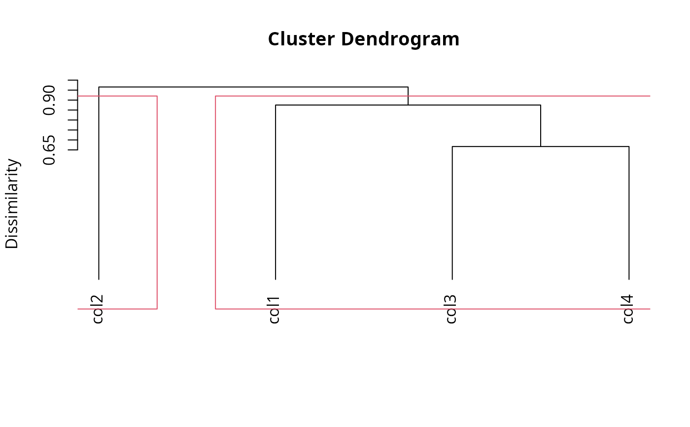cut3 <- cut_tree(tree3, k = 2)
cut3
#> $scores
#>      cluster_1    cluster_2
#> 1  -0.57975807  0.798023987
#> 2   0.35955426 -1.254465882
#> 3   0.91697780 -1.709962813
#> 4   0.25597952  0.166557223
#> 5   2.17073277  0.453523726
#> 6  -0.20067888 -0.964364009
#> 7   1.25304045 -0.302185721
#> 8  -0.88462772  1.039862981
#> 9  -1.97938047  2.352957237
#> 10 -0.17328140 -1.283216658
#> 11 -0.83751009  0.921412428
#> 12  1.95944585  0.310903005
#> 13 -1.44854555 -0.234197444
#> 14 -1.42657435 -0.896717844
#> 15 -0.42177003 -0.125455236
#> 16  0.31897514 -0.656418991
#> 17 -0.48146972 -0.948589669
#> 18  1.38138429  0.426483568
#> 19 -0.24822105 -0.001764805
#> 20  0.36497170 -0.754880977
#> 21 -0.86458815 -1.047738159
#> 22  0.58617615  0.868179125
#> 23  0.13249049 -0.413348233
#> 24 -0.28522122 -0.671568654
#> 25  0.16247706 -1.528560062
#> 26 -0.20810595  1.140870308
#> 27  1.00372186 -1.472259342
#> 28 -0.27070975  1.216660076
#> 29  0.12961219 -1.320922607
#> 30 -1.32540739 -0.136449077
#> 31  0.84061791 -0.909647145
#> 32 -0.94376204  1.929881073
#> 33 -0.51910451  0.163522246
#> 34  1.81651631  0.526602907
#> 35 -0.24929267  1.396259650
#> 36 -1.53910567 -0.125181338
#> 37  1.23624313  1.126064077
#> 38  1.25356602 -1.837230153
#> 39  1.29069152 -1.254108613
#> 40  0.37441825  0.632222908
#> 41 -0.34850099 -0.083827258
#> 42  0.51359279 -0.201139116
#> 43  1.13794604  0.094421942
#> 44  0.36540046  2.478704709
#> 45 -0.66564981 -1.285768725
#> 46  0.41184715 -0.568059271
#> 47  0.39301471  0.231860079
#> 48  0.22566810  0.374470060
#> 49  0.26789425 -1.640458691
#> 50  1.67375826 -0.153980124
#> 51 -1.24315302 -0.605182264
#> 52 -2.72259173 -1.284466321
#> 53 -2.04355042 -1.175136434
#> 54  0.83390951  1.293578076
#> 55  1.05711763  0.855835562
#> 56 -0.53854746 -2.575042455
#> 57 -0.69394250 -0.900025690
#> 58  0.81168918  0.886209006
#> 59  0.27789467  0.808966767
#> 60  0.51701388  0.896340922
#> 61  0.91155520 -1.437137188
#> 62 -1.63933737  0.322616676
#> 63  1.41214490 -0.578895302
#> 64  0.81265668 -0.978124905
#> 65  1.02307006  0.558315197
#> 66  0.03495272 -0.208072830
#> 67  0.55453391 -1.334803417
#> 68  1.33127729 -1.047975965
#> 69 -0.30677711  0.513230173
#> 70 -0.66871499 -0.335889343
#> 71 -0.82983283 -1.278766968
#> 72  0.61695755  0.217041912
#> 73  1.42924715 -1.853519134
#> 74 -1.11523114  1.357033554
#> 75  0.02145295 -1.278598610
#> 76  2.85062676 -1.703215064
#> 77 -1.93988909 -0.803403572
#> 78  0.33417271  0.418723431
#> 79  0.92702720 -1.771211916
#> 80 -0.95806587 -2.277864959
#> 
#> $scores_cor_matrix
#> NULL
#> 
#> $vars
#>   cluster variable squared_association association
#> 1       1     col2           1.0000000   1.0000000
#> 2       2     col4           0.5367779   0.7326513
#> 3       2     col3           0.5097153   0.7139435
#> 4       2     col1           0.4113961  -0.6414017
#> 
#> $vars_cor_matrix
#> $vars_cor_matrix$cluster_1
#> NULL
#> 
#> $vars_cor_matrix$cluster_2
#> NULL
#> 
#> 
#> $cluster
#> col1 col2 col3 col4 
#>    2    1    2    2 
#> 
#> $H
#> cluster_1 cluster_2 
#>  1.000000  1.457889 
#> 
#> $Hprop
#> [1] 0.3850692
#> 
#> $size
#> cluster_1 cluster_2 
#>         1         3 
#> 
#> $k
#> [1] 2
#> 
#> $call
#> cut_tree(x = tree3, k = 2)
#> 
#> $method
#> [1] "cut_tree"
#>

Partition a tree from `build_tree()`

Usage

Arguments

Value

See also

Examples