Add confidence intervals for power estimates
add_power_ci.RdCalculates and adds confidence intervals for power estimates to objects returned by power().
The confidence interval quantifies uncertainty about the true power parameter.
Usage
add_power_ci(x, ci_level = 0.95, method = c("wilson", "exact"))Arguments
- x
(data.frame)
A data frame returned bypower(), containing columnspowerandnsims.- ci_level
(Scalar numeric:
0.95;(0,1))
The confidence interval level.- method
(Scalar character:
"wilson";c("wilson", "exact"))
Method for computing confidence intervals. One of"wilson"(default) or"exact".
Value
The input data frame with additional columns:
| Name | Description |
power_ci_lower | Lower bound of confidence interval. |
power_ci_upper | Upper bound of confidence interval. |
and added attribute "ci_info" containing the method description, method name and confidence level.
Details
Power estimation via simulation is a binomial proportion problem. The confidence interval answers: "What is the plausible range of true power values given my simulation results?"
Let \(\pi\) denote the true power value, \(\hat{\pi} = x/n\) denote the observed power value, \(n\) denote the number of simulations, and \(x = \text{round}(\hat{\pi} \cdot n)\) denote the number of rejections. Two methods are available.
Wilson Score Interval
The Wilson score interval is derived from inverting the score test. Starting with the inequality
$$ \left| \frac{\hat{\pi}-\pi}{\sqrt{\pi(1-\pi)/n}} \right| \le z_{1-\alpha/2}, $$
and solving the resulting quadratic for \(\pi\) yields
$$ \frac{\hat{\pi}+\frac{z^2}{2n} \pm z \sqrt{\frac{\hat{\pi}(1-\hat{\pi})}{n}+\frac{z^2}{4n^2}}}{1+\frac{z^2}{n}}, $$
with \(z = z_{1-\alpha/2}\) and \(\hat{\pi} = x/n\).
Clopper-Pearson Interval
The Clopper-Pearson exact interval inverts the binomial test via Beta quantiles. The bounds \((\pi_L, \pi_U)\) satisfy:
$$P(X \geq x \mid \pi = \pi_L) = \alpha/2$$ $$P(X \leq x \mid \pi = \pi_U) = \alpha/2$$
With \(x\) successes in \(n\) trials,
$$\pi_L = B^{-1}\left(\frac{\alpha}{2}; x, n-x+1\right)$$ $$\pi_U = B^{-1}\left(1-\frac{\alpha}{2}; x+1, n-x\right)$$
where \(B^{-1}(q; a, b)\) is the \(q\)-th quantile of \(\text{Beta}(a, b)\).
This method guarantees at least nominal coverage but is conservative (intervals are wider than necessary).
Approximate parametric tests
When power is computed using approximate parametric tests (see simulated()), the power estimate and confidence/prediction intervals apply to the Monte Carlo test power \(\mu_K = P(\hat{p} \leq \alpha)\) rather than the exact test power \(\pi = P(p \leq \alpha)\).
These quantities converge as the number of datasets simulated under the null hypothesis \(K\) increases.
The minimum observable p-value is \(1/(K+1)\), so \(K > 1/\alpha - 1\) is required to observe any rejections.
For practical accuracy, we recommend choosing \(\text{max}(5000, K \gg 1/\alpha - 1)\) for most scenarios.
For example, if \(\alpha = 0.05\), use simulated(nsims = 5000).
References
Newcombe RG (1998). “Two-sided confidence intervals for the single proportion: comparison of seven methods.” Statistics in Medicine, 17(8), 857–872. ISSN 0277-6715, 1097-0258, doi:10.1002/(SICI)1097-0258(19980430)17:8<857::AID-SIM777>3.0.CO;2-E . ,
Wilson EB (1927). “Probable Inference, the Law of Succession, and Statistical Inference.” Journal of the American Statistical Association, 22(158), 209–212. ISSN 0162-1459, 1537-274X, doi:10.1080/01621459.1927.10502953 . ,
Clopper CJ, Pearson ES (1934). “THE USE OF CONFIDENCE OR FIDUCIAL LIMITS ILLUSTRATED IN THE CASE OF THE BINOMIAL.” Biometrika, 26(4), 404–413. ISSN 0006-3444, 1464-3510, doi:10.1093/biomet/26.4.404 .
Examples
#----------------------------------------------------------------------------
# add_power_ci() examples
#----------------------------------------------------------------------------
library(depower)
set.seed(1234)
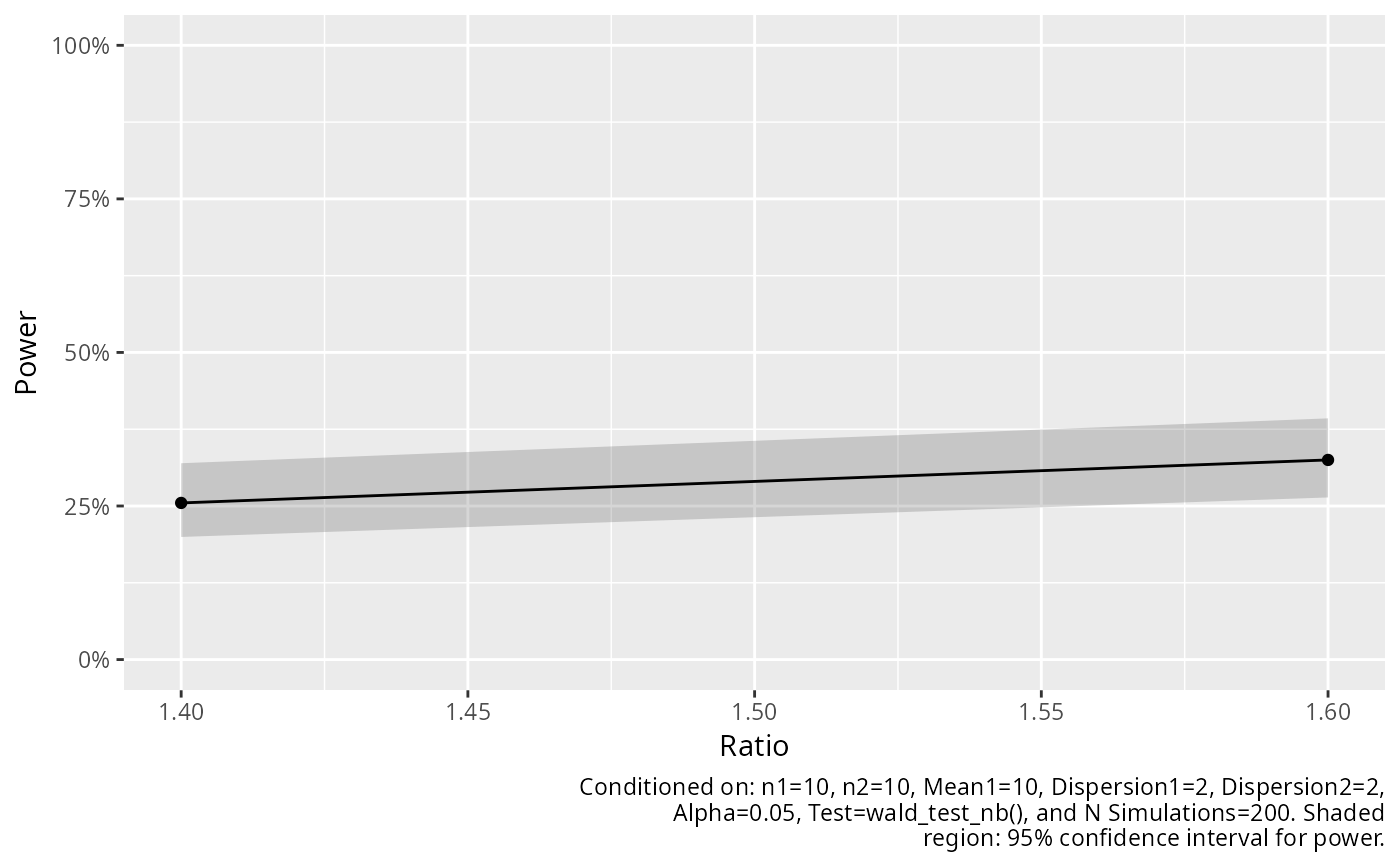
x <- sim_nb(
n1 = 10,
mean1 = 10,
ratio = c(1.4, 1.6),
dispersion1 = 2,
nsims = 200
) |>
power(wald_test_nb())
# Compare methods
add_power_ci(x, method = "wilson")
#> # A tibble: 2 × 14
#> n1 n2 mean1 mean2 ratio dispersion1 dispersion2 distribution nsims test
#> <dbl> <dbl> <dbl> <dbl> <dbl> <dbl> <dbl> <chr> <dbl> <chr>
#> 1 10 10 10 14 1.4 2 2 Independent… 200 wald…
#> 2 10 10 10 16 1.6 2 2 Independent… 200 wald…
#> # ℹ 4 more variables: alpha <dbl>, power <dbl>, power_ci_lower <dbl>,
#> # power_ci_upper <dbl>
add_power_ci(x, method = "exact")
#> # A tibble: 2 × 14
#> n1 n2 mean1 mean2 ratio dispersion1 dispersion2 distribution nsims test
#> <dbl> <dbl> <dbl> <dbl> <dbl> <dbl> <dbl> <chr> <dbl> <chr>
#> 1 10 10 10 14 1.4 2 2 Independent… 200 wald…
#> 2 10 10 10 16 1.6 2 2 Independent… 200 wald…
#> # ℹ 4 more variables: alpha <dbl>, power <dbl>, power_ci_lower <dbl>,
#> # power_ci_upper <dbl>
# 99% confidence interval
add_power_ci(x, ci_level = 0.99)
#> # A tibble: 2 × 14
#> n1 n2 mean1 mean2 ratio dispersion1 dispersion2 distribution nsims test
#> <dbl> <dbl> <dbl> <dbl> <dbl> <dbl> <dbl> <chr> <dbl> <chr>
#> 1 10 10 10 14 1.4 2 2 Independent… 200 wald…
#> 2 10 10 10 16 1.6 2 2 Independent… 200 wald…
#> # ℹ 4 more variables: alpha <dbl>, power <dbl>, power_ci_lower <dbl>,
#> # power_ci_upper <dbl>
# Plot with shaded region for confidence interval of the power estimate.
add_power_ci(x) |>
plot()