Add Bayesian posterior predictive intervals for power estimates

Calculates and adds Bayesian posterior predictive intervals for power estimates in objects returned by power(). The posterior predictive interval quantifies the expected range of power estimates from a future simulation study.

Usage

add_power_pi(x, future_nsims = NULL, pi_level = 0.95, prior = c(1, 1))

Arguments

x: (data.frame)
A data frame returned by power(), containing columns power and nsims.
future_nsims: (Scalar integer or NULL: NULL; [2, Inf))
Number of simulated data sets in the future power estimate study. If NULL (default), uses the same number as the original study (nsims).
pi_level: (Scalar numeric: 0.95; (0,1))
The posterior predictive interval level.
prior: (Numeric vector of length 2: c(1, 1); each (0, Inf))
Parameters $(\alpha, \beta)$ for the Beta prior on true power. Default c(1, 1) is the uniform prior. Use c(0.5, 0.5) for the Jeffreys prior.

Value

The input data frame with additional columns:

Name	Description
`power_pi_mean`	Predictive mean of future power estimate.
`power_pi_lower`	Lower bound of posterior predictive interval.
`power_pi_upper`	Upper bound of posterior predictive interval.

and added attribute "pi_info" containing the method description, method name, level, prior values, and future simulation count.

Details

Power estimation via simulation is a binomial proportion problem. The posterior predictive interval answers: "If I run a new simulation study with $m$ simulations, what range of power estimates might I observe?"

Let $\pi$ denote the true power value, $\hat{\pi} = x/n$ denote the observed power value, $n$ denote the number of simulations, and $x = \text{round}(\hat{\pi} \cdot n)$ denote the number of rejections. With a $\text{Beta}(\alpha, \beta)$ prior on the true power $\pi$, the posterior after observing $x$ successes in $n$ trials is:

$$ \pi \mid X = x \sim \text{Beta}(\alpha + x, \beta + n - x). $$

The posterior predictive distribution for $Y$, the number of successes in a future study with $m$ trials, is Beta-Binomial:

$$ Y \mid X = x \sim \text{BetaBinomial}(m, \alpha + x, \beta + n - x). $$

The posterior predictive interval is constructed from quantiles of this distribution, expressed as proportions $Y/m$.

The posterior predictive mean and variance of $\hat{\pi}_{\text{new}} = Y/m$ are: $$ \begin{aligned} E[\hat{\pi}_{\text{new}} \mid X = x] &= \frac{\alpha + x}{\alpha + \beta + n} \\ \text{Var}[\hat{\pi}_{\text{new}} \mid X = x] &= \frac {(\alpha + x)(\beta + n - x)(\alpha + \beta + n + m)} {m (\alpha + \beta + n)^{2} (\alpha + \beta + n + 1)}. \end{aligned} $$

Argument `future_nsims`

The argument future_nsims allows you to estimate prediction interval bounds for a hypothetical future study with different number of simulations. Note that a small initial number for nsims results in substantial uncertainty about the true power. A correspondingly large number of future simulations future_nsims will more precisely estimate the true power, but the past large uncertainty is still carried forward. Therefore you still need an adequate number of simulations nsims in the original study, not just more in the replication future_nsims, to ensure narrow prediction intervals.

Approximate parametric tests

When power is computed using approximate parametric tests (see simulated()), the power estimate and confidence/prediction intervals apply to the Monte Carlo test power $\mu_K = P(\hat{p} \leq \alpha)$ rather than the exact test power $\pi = P(p \leq \alpha)$. These quantities converge as the number of datasets simulated under the null hypothesis $K$ increases. The minimum observable p-value is $1/(K+1)$, so $K > 1/\alpha - 1$ is required to observe any rejections. For practical accuracy, we recommend choosing $\text{max}(5000, K \gg 1/\alpha - 1)$ for most scenarios. For example, if $\alpha = 0.05$, use simulated(nsims = 5000).

References

Gelman A, Carlin JB, Stern HS, Dunson DB, Vehtari A, Rubin DB (2013). Bayesian data analysis, Texts in statistical science series, Third edition edition. CRC Press, Taylor & Francis Group. ISBN 9781439840955.

Examples

#----------------------------------------------------------------------------
# add_power_pi() examples
#----------------------------------------------------------------------------
library(depower)

set.seed(1234)
x <- sim_nb(
  n1 = 10,
  mean1 = 10,
  ratio = c(1.4, 1.6),
  dispersion1 = 2,
  nsims = 200
) |>
  power(wald_test_nb())

# Add posterior predictive intervals
# default: predict for same number of simulations
add_power_pi(x)
#> # A tibble: 2 × 15
#>      n1    n2 mean1 mean2 ratio dispersion1 dispersion2 distribution nsims test 
#>   <dbl> <dbl> <dbl> <dbl> <dbl>       <dbl>       <dbl> <chr>        <dbl> <chr>
#> 1    10    10    10    14   1.4           2           2 Independent…   200 wald…
#> 2    10    10    10    16   1.6           2           2 Independent…   200 wald…
#> # ℹ 5 more variables: alpha <dbl>, power <dbl>, power_pi_mean <dbl>,
#> #   power_pi_lower <dbl>, power_pi_upper <dbl>

# Compare posterior predictive interval width across different future
# study sizes
add_power_pi(x, future_nsims = 100)  # wider
#> # A tibble: 2 × 15
#>      n1    n2 mean1 mean2 ratio dispersion1 dispersion2 distribution nsims test 
#>   <dbl> <dbl> <dbl> <dbl> <dbl>       <dbl>       <dbl> <chr>        <dbl> <chr>
#> 1    10    10    10    14   1.4           2           2 Independent…   200 wald…
#> 2    10    10    10    16   1.6           2           2 Independent…   200 wald…
#> # ℹ 5 more variables: alpha <dbl>, power <dbl>, power_pi_mean <dbl>,
#> #   power_pi_lower <dbl>, power_pi_upper <dbl>
add_power_pi(x, future_nsims = 1000) # narrower
#> # A tibble: 2 × 15
#>      n1    n2 mean1 mean2 ratio dispersion1 dispersion2 distribution nsims test 
#>   <dbl> <dbl> <dbl> <dbl> <dbl>       <dbl>       <dbl> <chr>        <dbl> <chr>
#> 1    10    10    10    14   1.4           2           2 Independent…   200 wald…
#> 2    10    10    10    16   1.6           2           2 Independent…   200 wald…
#> # ℹ 5 more variables: alpha <dbl>, power <dbl>, power_pi_mean <dbl>,
#> #   power_pi_lower <dbl>, power_pi_upper <dbl>

# Use Jeffreys prior instead of uniform
add_power_pi(x, prior = c(0.5, 0.5))
#> # A tibble: 2 × 15
#>      n1    n2 mean1 mean2 ratio dispersion1 dispersion2 distribution nsims test 
#>   <dbl> <dbl> <dbl> <dbl> <dbl>       <dbl>       <dbl> <chr>        <dbl> <chr>
#> 1    10    10    10    14   1.4           2           2 Independent…   200 wald…
#> 2    10    10    10    16   1.6           2           2 Independent…   200 wald…
#> # ℹ 5 more variables: alpha <dbl>, power <dbl>, power_pi_mean <dbl>,
#> #   power_pi_lower <dbl>, power_pi_upper <dbl>

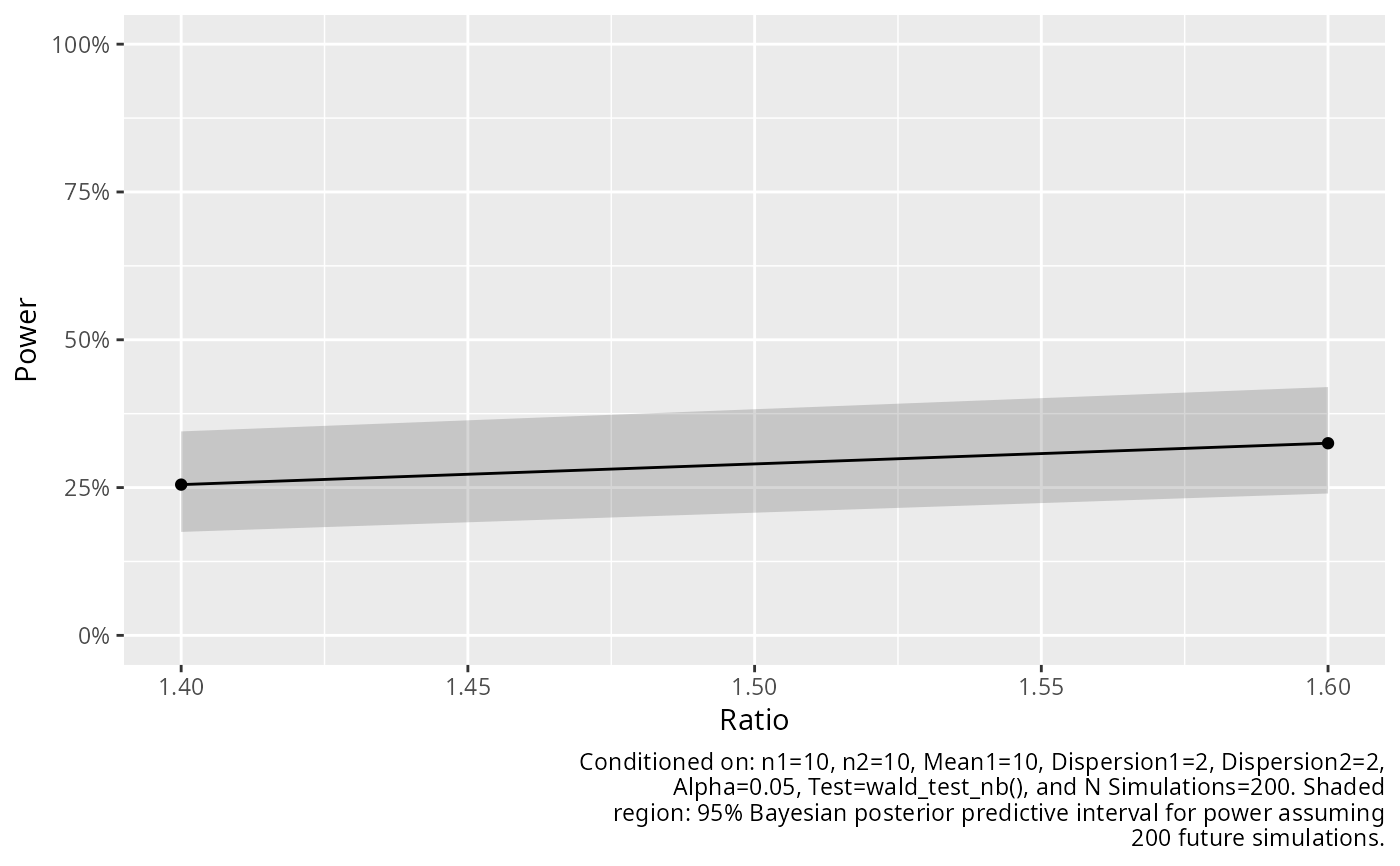
# Plot with shaded region for prediction interval of the power estimate.
add_power_pi(x) |>
  plot()